typhoon haiyan case study physics and maths tutor

• 0 Shopping Cart

Typhoon Haiyan Case Study

What were the primary and secondary effects of Typhoon Haiyan? What were the immediate and long-term responses?

What were the primary effects of Typhoon Haiyan?

Typhoon Haiyan, a category five typhoon, struck the Philippines, close to Tacloban on 8th November, 2013 at 4.40 am. The tropical storm originated in the northwest Pacific Ocean. It is one of the most powerful typhoons to affect the Philippines. Wind speeds of 314 kilometres per hour (195 miles per hour) were recorded.

Typhoon Haiyan

The primary effects of Typhoon Haiyan were:

• strong winds battered homes
• people were made homeless, particularly around Western and Eastern Visayas
• electric was interrupted
• airport badly damaged
• roads were blocked by fallen trees and other debris
• Leyte and Tacloban experienced a 5-metre storm surge, and 400mm of rainfall flooded an area of up to 1km inland
• 90% of Tacloban was destroyed
• 6190 people died
• 29,000 people were injured
• 4.1 million people were made homeless
• 14.1 million people affected
• The overall cost of damage was around $12 billion
• 1.1 million tonnes of crops destroyed
• 1.1 million houses damaged
• 1 million farmers and 600,000 hectares of farmland affected

The strong winds battered homes and even the evacuation centre buildings. Those made homeless were mainly in the Western and Eastern Visayas. Power was interrupted, the airport was severely damaged, and trees and debris blocked roads. Leyte and Tacloban had a five-metre storm surge, and 400 millimetres of heavy rainfall flooded one kilometre inland. Ninety per cent of the city of Tacloban was destroyed.

Debris lines the streets of Tacloban, Leyte island. This region was the worst affected by the typhoon, causing widespread damage and loss of life. Caritas responds by distributing food, shelter, hygiene kits and cooking utensils. (Photo: Eoghan Rice – Trócaire / Caritas)

Although the harvest season was over, rice and seed stocks were squandered in the storm surges, leading to a $53 million US dollars loss.

Over one-third of farmers and fishers lost their income, leading to a total loss of $724 million.

What were the secondary effects?

Social effects

• Infection and diseases spread, mainly due to contaminated surface and ground water.
• Survivors fought for food and supplies. Eight people died in a stampede for food supplies.
• Power supplies were cut off for months in some areas.
• Education was disrupted as many schools were destroyed.
• Seawater, chemicals and sewerage contaminated surface and groundwater.

Economic effects

• An oil tanker ran aground, causing an 800,000-litre oil leak that contaminated fishing waters.
• The airport was badly damaged and roads were blocked by debris and trees.
• Looting was rife, due to the lack of food and supplies.
• Rice prices had risen by nearly 12% by 2014.

Environmental effects

• The leak from the oil barge led to ten hectares of mangroves being contaminated.
• Flooding caused landslides.

What were the immediate responses?

The government issued a televised warning to people to prepare and evacuate.

Eight hundred thousand people were evacuated following a televised warning by the president. Many people found refuge in a stadium in Tacloban. However, many people died when it was flooded. The government provided essential equipment and medical supplies. A curfew was introduced two days after the typhoon to reduce looting.

Over 1,200 evacuation centres were set up to help the homeless.

Three days after the storm, the main airport was reopened, and emergency aid arrived. Power was restored in some regions after a week. One million food packs and 250,000 litres of water were distributed within two weeks.

Over $1.5 billion of foreign aid was pledged. Thirty-three countries and international organisations promised help, with rescue operations and an estimated US $ 88.871 million.

What were the long-term responses?

A cash for work programme paid people to clear debris and rebuild Tacloban.

The international charity organisation Oxfam replaced fishing boats.

Build Back Better is the government’s response to the typhoon. Launched in 2014, it intended to upgrade damaged buildings to protect them from future disasters. They have also set up a no-build zone along the coast in Eastern Visayas, a new storm surge warning system has been developed, and mangroves replanted to absorb future storm surges.

Premium Resources

Please support internet geography.

If you've found the resources on this page useful please consider making a secure donation via PayPal to support the development of the site. The site is self-funded and your support is really appreciated.

Hurricane Michael

Topic home, typhoon jebi case study, share this:.

• Click to share on Twitter (Opens in new window)
• Click to share on Facebook (Opens in new window)
• Click to share on Pinterest (Opens in new window)
• Click to email a link to a friend (Opens in new window)
• Click to share on WhatsApp (Opens in new window)
• Click to print (Opens in new window)

If you've found the resources on this site useful please consider making a secure donation via PayPal to support the development of the site. The site is self-funded and your support is really appreciated.

Search Internet Geography

Top posts and pages.

Latest Blog Entries

Pin It on Pinterest

• Click to share
• Print Friendly

Article  

• Volume 22, issue 10
• NHESS, 22, 3285–3307, 2022
• Peer review
• Related articles

Sensitivity of simulating Typhoon Haiyan (2013) using WRF: the role of cumulus convection, surface flux parameterizations, spectral nudging, and initial and boundary conditions

Rafaela jane delfino, gerry bagtasa, kevin hodges, pier luigi vidale.

Typhoon (TY) Haiyan was one of the most intense and highly destructive tropical cyclones (TCs) to affect the Philippines. As such, it is regarded as a baseline for extreme TC hazards. Improving the simulation of such TCs will not only improve the forecasting of intense TCs but will also be essential in understanding the potential sensitivity of future intense TCs with climate change. In this study, we investigate the effects of model configuration in simulating TY Haiyan using the Weather Research Forecasting (WRF) Model. Sensitivity experiments were conducted by systematically altering the choice of cumulus schemes, surface flux options, and spectral nudging. In addition to using the European Centre for Medium-Range Weather Forecasts Reanalysis fifth-generation (ERA5) single high-resolution realization as initial and boundary conditions, we also used 4 of the 10 lower-resolution ERA5 data assimilation system (EDA) ensemble members as initial and boundary conditions. Results indicate a high level of sensitivity to cumulus schemes, with a trade-off between using Kain–Fritsch and Tiedtke schemes that have not been mentioned in past studies of TCs in the Philippines. The Tiedtke scheme simulates the track better (with a lower mean direct positional error, DPE, of 33 km), while the Kain–Fritsch scheme produces stronger intensities (by 15 hPa minimum sea level pressure). Spectral nudging also resulted in a reduction in the mean DPE by 20 km, and varying the surface flux options resulted in the improvement of the simulated maximum sustained winds by up to 10 m s −1 . Simulations using the EDA members initial and boundary conditions revealed low sensitivity to the initial and boundary conditions, having less spread than the simulations using different parameterization schemes. We highlight the advantage of using an ensemble of cumulus parameterizations to take into account the uncertainty in the track and intensity of simulating intense tropical cyclones.

• Article (PDF, 13394 KB)
• Supplement (1667 KB)
• Article (13394 KB)

Delfino, R. J., Bagtasa, G., Hodges, K., and Vidale, P. L.: Sensitivity of simulating Typhoon Haiyan (2013) using WRF: the role of cumulus convection, surface flux parameterizations, spectral nudging, and initial and boundary conditions, Nat. Hazards Earth Syst. Sci., 22, 3285–3307, https://doi.org/10.5194/nhess-22-3285-2022, 2022.

As a country of 109 million people over more than 7000 islands, the Philippines is considered one of the most natural-hazard-prone countries in the world (Brucal et al., 2020) and is ranked in the top five of all countries in terms of exposure to climate-related risks (Eckstein et al., 2020). One of the most important hazards the Philippines is exposed to is tropical cyclones (TCs). TCs bring intense winds, extreme precipitation, and storm surges that affect a large portion of the Philippine population (Bagtasa, 2017; Lyon and Camargo, 2009). Due to its location in the western North Pacific Ocean, where TC formation is conducive all year, the Philippines is exposed to an average 10 landfalling TCs annually (Cinco et al., 2016). Since 1990, TCs in the Philippines have resulted in up to half of the total losses from all natural disasters, amounting to about USD 20 billion in damages (Brucal et al., 2020) and an annual average death toll of 885 with estimated accumulated deaths due to TCs of approximately 30 000 from 1980 to 2013 (Yonson et al., 2016). It is estimated that about 5 million people are affected annually or over 570 000 are affected on average per destructive TC (Brucal et al., 2020).

One of the strongest typhoons that made landfall in the Philippines in recent history is Typhoon (TY) Haiyan (locally named “Yolanda”), which is considered the second costliest Philippine TC since 1990 (EM-DAT, 2020) and one of the deadliest since the 1970s (Cinco et al., 2016; Lander et al., 2014; Lagmay et al., 2015). TY Haiyan was a category-5 super typhoon that claimed the lives of at least 7300 people, most of them from drowning due to the devastating 5 to 7 m high storm surge and coastal inundation (Soria et al., 2016). It also affected more than 16 million people (NDRRMC, 2014) and caused an estimated USD 5–15 billion worth of damage, particularly in agriculture and critical infrastructure (Brucal et al., 2020). Comiso et al. (2015) found that TY Haiyan coincided with the warmest sea surface temperature (SST) observed over the Pacific warm-pool region, which may have contributed to its intense nature. This relation between intense TCs and warmer tropical SSTs has also been found in the Atlantic (Emanuel, 2005) and suggests that continuous warming may lead to more intense TCs in the future. Consistently, an increasing trend in intense TC frequency affecting the Philippines since the 1970s has been observed (Cinco et al., 2016; Comiso et al., 2015). TC rainfall is also expected to increase in the future as TCs intensify (IPCC, 2021; Patricola and Wehner, 2018), potentially increasing the risk of flooding and landslides. Given TY Haiyan's intensity and impacts, it is regarded as a benchmark for an intense and destructive TC. Hence, it is important to test how well it can be simulated in current models in the present climate and the TC sensitivities to model formulation.

While global climate models (GCMs) are very useful for looking at the changes in TC activity under different climate change scenarios (e.g., frequency, intensity, genesis from a climatological and global/regional perspective) (Gallo et al., 2019; Patricola and Wehner, 2018) and some advances have been made in the past few decades in the use of global convection-permitting models (Judt et al., 2021), previous studies still demonstrate the need for (convection-resolving/convection-permitting) limited area models (LAMs) to better simulate the processes relevant to the TC formation and development as well as their properties, particularly the most intense ones (e.g., Walsh et al., 2015). In consideration of the computational cost in resolving important TC processes, the use of LAMs is a valuable and complementary approach to using GCMs in investigating the potential changes in TCs in the future. One such LAM is the Weather Research and Forecasting (WRF) Model (Skamarock et al., 2008), developed by the National Center for Atmospheric Research (NCAR), which is used as both numerical weather prediction LAM and regional climate model (RCM). WRF is currently used for operational forecasting in the Philippines by the country's meteorological office – Philippine Atmospheric, Geophysical and Astronomical Services Administration (PAGASA) (Flores, 2019; Aragon and Pura, 2016) – and also used in hindcast simulation and sensitivity studies of TC track and intensity (Spencer et al., 2012; Islam et al., 2015; Lee and Wu, 2018) and associated rainfall (Cruz and Narisma, 2016). It has also been used as an RCM to simulate TC activity in the western North Pacific (WNP) basin (Shen et al., 2017) and several TCs in the North Atlantic over a 13-year period in a convection-permitting model under current and future climate conditions (Gutmann et al., 2018). It has also been used as LAM in simulating specific TC cases with future GCM forcings as initial and lateral boundary conditions in other TC basins (Lackmann, 2015; Parker et al., 2018; Patricola and Wehner, 2018).

WRF has also gained considerable popularity in recent years and has been used for TC simulations (Islam et al., 2015). Efforts are being made to identify the optimum parameterization schemes and to customize the WRF-ARW model for TC hindcast simulations. For instance, past numerical weather prediction (NWP) LAM studies of western North Pacific TCs, including TY Haiyan, show the cumulus (CU) convection scheme as having the most influence on its intensity over other model parameters such as the planetary boundary layer (PBL) and/or microphysics schemes (Islam et al., 2014; Di et al., 2019). In particular, the Kain–Fritsch (KF) (Kain, 2004) cumulus convection scheme has been found to produce the best TC tracks and wind intensity estimates (Zhang et al., 2011; Spencer et al., 2012; Prater and Evans, 2002; Mohandas and Ashrit, 2014). Furthermore, the often-selected KF scheme was shown to be also sensitive to model resolution (Li et al., 2018). However, the use of the KF scheme has also shown certain limitations. A study by Torn and Davis (2012) found that the KF scheme produces larger TC track biases than the Tiedtke (TK) cumulus convection scheme.

Other than the said parameterization schemes, improvements in simulations of TC intensity have also been found to be influenced by the surface flux options (Kueh et al., 2019). Some other studies related to the sensitivity of WRF model choices can be found, i.e., spectral nudging (Moon et al., 2018) and initial and boundary conditions (Islam et al., 2015). Previous work has explored the sensitivity of TC simulations in WRF to initial condition datasets, i.e., from different reanalysis data (e.g., Mohanty et al., 2010) and initial condition time (e.g., Mohanty et al., 2010; Shepherd and Walsh, 2017). Shepherd and Walsh (2017) showed that trajectories can be sensitive to initial condition time; however, they are more sensitive to the CU parameterization. Mohanty et al. (2010) demonstrated that simulated intensity and vorticity maxima are sensitive to the chosen initial and boundary condition dataset. Alternatively, nudging could be applied to the model until TC genesis, which would constrain the model to be more consistent with observations. Mori et al. (2014) applied spectral nudging in several runs in its hindcast WRF simulations for Typhoon Haiyan and found that when applied, there is some bias in the simulated track primarily at landfall, but it simulated reasonable intensities. Kueh et al. (2019) also performed several experiments with and without nudging at 3 km resolution and found that nudging produced smaller track errors than the simulations without. They also found small differences in the TC intensity and structure in the experiments with and without nudging. Cha et al. (2011) suggested that continued spectral nudging can suppress TC intensification. Shen et al. (2017), although using WRF as an RCM in investigating the effect of spectral nudging in inter-annual and seasonal variability of TC activity in East Asia, suggested that the nudging has an impact in reproducing TC activity. However, there are issues concerning the impact of nudging strength on model internal variability (Glisan et al., 2013). In this paper, we revisit the hindcast simulation of TY Haiyan using WRF as NWP LAM and assess its sensitivity to model formulation and the driving initial and boundary conditions, in preparation for pseudo-global warming and CMIP6 climate projection experiment studies. This study builds on the work of Islam et al. (2015), who assessed the effects of different combinations of the planetary boundary layer, microphysics, and cumulus convection scheme using WRF but found substantial underestimation of TY Haiyan's intensity regardless of the sensitivity to physics parameterization; Li et al. (2018), who used WRF to look at the effects of the cumulus parameterization at different resolutions (9–2 km) and found that the most effective resolution to simulate TY Haiyan with no cumulus parameterization or a revised KF scheme is at 2 and 4 km resolution, respectively; and that of Kueh et al. (2019), who looked at the influence of the different surface flux options in simulating TY Haiyan's intensity using one cumulus convection scheme and found that a better representation of surface flux formulas improved the simulated intensity in WRF. Here, we investigate the effects of the different combinations of model cumulus convection schemes, spectral nudging, and surface flux options on the TY Haiyan track, intensity, and rainfall hindcast simulations.

Improving the representation of intense TCs like Haiyan in LAMs such as WRF is also essential for simulations of such TCs in different future climate change scenarios to provide credible impact assessments and useful for simulating TC cases under different climate conditions, e.g., pre-industrial or future (Parker et al., 2018; Patricola and Wehner, 2018; Chen et al., 2020). From this study the best combination is determined, which will then be used for investigating the effects of future climate change on TY Haiyan and other TC cases. The associated storm surge of TY Haiyan (Mori et al., 2014; Nakamura et al., 2016; and Takayabu et al., 2015) is not considered here. Model parameterization scheme sensitivity studies that assess the simulation of TCs will also provide guidance to future TC modeling studies (Villafuerte et al., 2021).

This study seeks to contribute to sensitivity studies with a particular focus on the Philippines by assessing the skill and sensitivity of a TC case study using a mesoscale NWP LAM model. In particular, it aims to study the influence of the combination of cumulus convection scheme, the different surface flux options for the different TC characteristics, and the use of spectral nudging. This study adds on existing literature by looking at the effects of cumulus convection schemes combined with different flux options and spectral nudging. Specifically, it aims to address the following questions.

How sensitive are the TY Haiyan hindcast simulations to convective schemes, surface flux options, and spectral nudging?

How sensitive are the simulated track and intensity of TY Haiyan to the uncertainty in the initial and boundary conditions?

The results will provide valuable information for regional climate downscaling of intense TCs, which can be used in evaluating the sensitivity of future TCs in climate change simulations. Section 2 provides a description of the methodology. Then the paper continues with the results of the sensitivity experiments followed by the discussion, and finally Sect. 4 provides a summary of the findings and recommendations for future work.

2.1  Case study: Typhoon Haiyan brief description

Typhoon Haiyan originated from an area of low pressure near the Federated States of Micronesia (5.8 ∘  N, 157.2 ∘  E) on 2 November 2013 and moved westward, forming into a tropical storm on 2 November 2013. Typhoon Haiyan formed in an environment with a significantly high SSTs (peaking at 30.1  ∘ C in November 2013), which was considered the highest observed during the period between 1981 and 2014 in the warm-pool region (Comiso et al., 2015). It then rapidly intensified into a TY on 5 November at 6.9 ∘  N, 142.9 ∘  E, was classified as a category-5-equivalent super typhoon by the Joint Typhoon Warning Center (JTWC), and was classified as a Typhoon by PAGASA, its highest classification at the time. It further intensified before making landfall on 7 November at 20:40 UTC. It traversed the central section of the Philippines and started to slowly weaken to a tropical depression on 11 November (JMA, 2013). Typhoon Haiyan claimed the lives of more than 7300 people, mostly due to the associated storm surge and coastal inundation. It is estimated to have caused USD 5–15 billion worth of direct damages in agriculture and infrastructure (Brucal et al., 2020) and affected more than 16 million people (NDRRMC, 2014).

2.2  Model description

Simulations were conducted using WRF version 3.8.1 (Skamarock et al., 2008), a non-hydrostatic numerical weather prediction LAM developed by the National Center for Atmospheric Research (NCAR). It is used for atmospheric research and operational forecasting and increasingly for regional climate research (Powers et al., 2017). The model includes a variety of physical parameterization schemes, including cumulus convection, microphysics, radiative transfer, planetary boundary layer, and land surface. The Advanced Research WRF (WRF-ARW) solver uses the Arakawa C grid as the computational grid and the Runge–Kutta third-order time integration schemes (MMML-NCAR, 2019). Skamarock et al. (2008) provides a more detailed description of the model specifications. PAGASA uses WRF for its operational forecasting over the Philippine Area of Responsibility (Flores, 2019; Aragon and Pura, 2016), and it is also used in studies simulating event-based TC-associated rainfall over the Philippines (Cruz and Narisma, 2016).

The land surface information comes from the 30 arcsec ( * 1  km) resolution Moderate Resolution Imaging Spectroradiometer (MODIS) satellite dataset with 20 global land use categories.

2.3  Initial and boundary conditions

The European Centre for Medium-Range Weather Forecasts (ECMWF) Reanalysis fifth-generation (ERA5) data are used for both the initial and boundary conditions. It is the latest generation of reanalysis products produced by ECMWF with a horizontal resolution of 31 km, hourly temporal resolution, and 137 vertical levels (Hersbach et al., 2020). ERA5 uses observations collected from satellites and in situ stations, which are quality controlled and assimilated using 4D-Var, a model based on the ECMWF's Integrated Forecast System (IFS) cycle 41r2.

Alongside the release of the ERA5 single-realization deterministic data from 1979 to the present, data from the Ensemble of Data Assimilations (EDA) system were also made available. The EDA system is a 10-member ensemble at a lower resolution than the deterministic data (60 km horizontal resolution and 3-hourly) (Hennermann, 2018). The EDA system provides estimates of analysis and short-range forecasts through one control and nine perturbed members, which provide background error estimates for the deterministic forecasts. This system allows for estimating uncertainty since it provides estimates of the analysis and short-range forecast. These are provided as an uncertainty measure, albeit with half the resolution of the reanalysis. To test the sensitivity to varying boundary conditions, simulations were also performed using four randomly selected representatives of the 10-member ERA5 EDA system. The selected ensemble members were used to test the sensitivity to different perturbed observations, sea surface temperature fields, and model physics (Isaksen et al., 2010).

2.4  Design of sensitivity experiments and analysis

In this study, the WRF–ARW model has been configured with two nested domains centered over the point of 18.3 ∘ latitude, 135 ∘ longitude. The outermost grid has 294×159 grid points with 25 km grid spacing, while the innermost domain has 745×550 grid points with 5 km grid spacing and 44 vertical eta levels, and the model top pressure level was set to 50 hPa. A two-way nesting is allowed for the interaction between the outer and inner domain. Specifically, for the outer domain, which is driven at the boundaries by ERA5, one-way nesting was used. For the inner domain, which is driven by the coarser domain, two-way nesting was used. The results shown in this paper are from the inner 5 km domain. This model resolution was chosen in favor of using supercomputing resources for the systematic testing of different parameterization schemes, as well as in consideration of additional simulations under future climate conditions.

Higher-resolution nested model configuration is widely used in numerical weather prediction and regional climate modeling. The main reason for this is because performing high-resolution simulation over very large areas (e.g., an entire major oceanic basin) is computationally too expensive (Kueh et al., 2019). The communication between the nested domains can be implemented using one-way or two-way nesting. One-way nesting means that the nested domains are run separately and sequentially starting with the outer domain; i.e., the model is first run for the outer domain to create an output which is used to supply the inner domain's boundary file. In a two-way nesting configuration, both domains are run simultaneously and interact with each other, so that the highest-possible-resolution information produced by the innermost domain affects the solutions over the overlapping area of the coarser domains. The input from the coarse outer domain is introduced through the boundary of the fine inner domain, while feedback to the coarse domain occurs all over the inner domain interior, as its values are replaced by combination of fine inner domain values (Alaka et al., 2022; Mure-Ravaud et al., 2019; Harris and Duran, 2010). We have used two-way nesting in the sensitivity runs, rather than one-way nesting, following recommended practice and previous studies that looked at sensitivities to physics parameterizations in WRF (Wu et al., 2019; Biswas et al., 2014; Li and Pu, 2009; Parker et al., 2017; Spencer et al., 2012; Bopape et al., 2021), studies that simulated Typhoon Haiyan in the Philippines (Li et al., 2018; Nakamura et al., 2016), and TC cases in other basins (Parker et al., 2018; Mittal et al., 2019; Reddy et al., 2021), among others. Studies of the differences in using one-way and two-way nesting in regional modeling have been the topic of multiple previous papers (e.g., Spencer et al., 2012; Matte et al., 2016; Raffa et al., 2021; Lauwaet et al., 2013; Harris and Durran, 2010; Chen et al., 2010; Gao et al., 2019). A comprehensive discussion on the differences and uncertainties associated with one-way or two-way nesting can also be found in Harris (2010). Studies such as those of Chen et al. (2010) and Gao et al. (2019) have shown that the use of one-way or two-way nesting showed little difference in the results, but some studies have shown that two-way nesting improves the simulations of TCs, e.g., Typhoon Parma in the Philippines (Spencer et al., 2012) and Typhoon Kai-tak (Wu et al., 2019). In addition, previous TC case studies in the Philippines have also used the two-way nesting configuration, e.g., Mori et al. (2014), Takayabu et al. (2015), and Nakamura et al. (2016). Other studies have also used two-way nesting in simulating TCs in other basins (Parker et al., 2018; Davis et al., 2008; Mittal et al., 2019; Reddy et al., 2021), as have studies that looked at sensitivity to different physics parameterizations (Wu et al., 2019; Biswas et al., 2014; Li and Pu, 2009). Two-way nesting is also used in operational TC forecasting (Mehra et al., 2019) and in the experimental Hurricane WRF system (Zhang et al., 2016) as well as in convection-permitting regional climate models (Lucas-Picher et al., 2021).

Different domain configurations were tested prior to selecting this particular configuration, with the current domain configuration having the track and intensity closest to that observed (Figs. S1–S5 in the Supplement). The domain configuration used in this study is used to have a common domain for different TC cases (other TC cases not included in this paper) to understand and have a more general set of conclusions on the response of TCs to future warming and to properly simulate the subtropical ridge/Western North Pacific Subtropical High (WNPSH).

In performing the experiments, WRF was run for a 180 h period from 00:00 UTC on 4 November 2013 to 12:00 UTC on 11 November 2013 to cover the main part of the life cycle of TY Haiyan. Simulations with different start times were conducted (Figs. S6–S7) to sample the different stages in TY Haiyan's lifetime and different initializations. Starting times tested include 4 November 2013 at 00:00 and 12:00 UTC, 5 November 2013 at 00:00 and 12:00 UTC, 6 November 2013 at 00:00 and 12:00 UTC, and 7 November 2013 at 00:00 UTC. The simulation that started on 4 November at 00:00 UTC was found to be optimal in terms of track and intensity; thus, the initialization time of all experiments was fixed at 4 November 2013 at 00:00 UTC. The longer lead time was also used to allow for the simulation of the early stages of development of Typhoon Haiyan. We considered the period covering 4 November 2013 at 00:00 UTC to 5 November 2013 at 12:00 UTC as the spin-up period. For the purposes of this paper, the analysis of the experiments covered only the 72 h period between 18:00 UTC on 5 November 2013 to 18:00 UTC on 8 November 2013 to cover TY Haiyan's mature stage.

Additional simulations using convection-permitting resolution (single domain, 4.5 km) were also performed and showed no significant change in simulated intensity from the configuration used here (not shown). The results shown in this paper are from the inner 5 km domain, with results of the outer 25 km domain shown in Fig. S8. The model domain setup is shown in Fig. 1.

Figure 1 Study domain setup. The outer 25 km resolution ( Δ x ) domain is bounded by 0–35 ∘  N and 100–170 ∘  E, while the inner 5 km resolution ( Δ x ) domain is bounded by 5–30 ∘  N and 115–150 ∘  E.

Convection is mostly simulated in models with resolution coarser than 10–5 km through the cumulus parameterization scheme. WRF's cumulus parameterization scheme simulates the effects of cumulus convection on heat, moisture, and precipitation at the sub-grid scale (Skamarock et al., 2008). The choice of cumulus parameterization schemes has an impact on WRF's ability to simulate the TC track, intensity, and structure (Zhang et al., 2011; Shepherd and Walsh, 2017; Parker et al., 2017). Only two schemes were investigated in this study – the KF scheme and TK scheme – the differences of which are summarized below in Table 1. The same physics parameterizations, including the cumulus scheme, were used in both inner and outer domains. PAGASA uses KF for its operational forecasting configurations (Flores, 2019). It has also often been used for TC simulation studies in the Philippines and has been found, in several studies, to be the best choice for simulating TC track and intensity (e.g., Sun et al., 2015; Li et al., 2018) and rainfall (e.g., Cruz and Narisma, 2016). The TK scheme, on the other hand, has been suggested to be the more appropriate cumulus scheme in tropical weather/climate applications of the WRF model (Parker et al., 2017). Torn and Davis (2012) showed an improvement in TC track simulations when using the TK scheme compared to the KF scheme. They stated that the TK scheme allows for more appropriate treatment of oceanic shallow convection due to a more active shallow convection scheme than that of the KF scheme. There was a 1 K temperature bias at 700 hPa in the KF scheme not present in the TK simulations, attributed to a lack of shallow convection in KF. These generated horizontal temperature gradients are associated with the wind biases affecting the TC tracks simulated with the KF scheme (Parker et al., 2018; Torn and Davis, 2012). In addition, according to Sun et al. (2015), deep convection in mass flux schemes, such as KF, produces large amounts of anvil clouds that warm the upper troposphere and cause latent heating south of the WNPSH that leads to the weakening of the WNPSH and the movement of the TCs northward. Li et al. (2018) investigated the sensitivities of the simulated tracks, intensities, and structures of Typhoon Haiyan to the use of a the revised KF scheme with varying resolutions from 9 to 2 km and found that the resulting simulations with the application of the revised KF (rKF) scheme are different at various resolutions. Cruz and Narisma (2016) also used the KF scheme in conducting sensitivity tests of TC-associated rainfall with different PBL and microphysics schemes in WRF.

Using a mass flux approach with downdraft removal and utilizing convective available potential energy (CAPE), KF is a deep and shallow convection sub-grid scheme that includes clouds, rain, ice, and snow detrainment and cloud persistence (Kain, 2004). Although KF can account for relatively small-scale processes that drive convection, it has inherent limitations in simulating shallow convection over tropical oceans (Parker et al., 2017). On the other hand, the TK scheme assumes that the moisture flux through the cloud base is equivalent to the surface moisture flux, as well as momentum transport, cloud detrainment, and ice detrainment (Tiedtke, 1989; Zhang et al., 2011). According to Parker et al. (2017), the TK scheme is more appropriate for simulating intense TCs in tropical oceans.

Table 1 Description of the cumulus schemes used in this study.

Sources: Adeniyi (2019), Torn and Davis (2012), and Shepherd and Walsh (2017).

Download Print Version | Download XLSX

Experiments were also conducted to examine the sensitivity to the available parameterizations for surface flux options. For TC applications, WRF-ARW provides three different formulations of aerodynamic roughness lengths of the surface momentum and scalar fields as surface flux options (isftcflx  =  0, 1, and 2) (see Kueh et al., 2019, for a detailed description of the differences between these options). It has been shown that surface fluxes can influence the model's ability to simulate TC intensity and structure (Green and Zhang, 2013; Kueh et al., 2019). For the default flux option (referred to here as sf0), the momentum roughness length is given as Charnock's (1955) expression plus a viscous term, following Smith (1988) – Eq. (1):

where α is the Charnock coefficient and v the kinematic viscosity of dry air, for which a constant value of 1.5 × 10 - 5  m 2  s −1 is used. A constant value of α =0.0185 is used for sf0.

Since the roughness length formulas in sf0 are demonstrably inconsistent with a substantial amount of research (Kueh et al., 2019), two more options were developed (hereinafter referred to as sf1 and sf2) (Kueh et al., 2019). Based on the findings that the drag coefficient (CD) seemed to level off at hurricane force wind speed (e.g., Powell et al., 2003; Donelan et al., 2004), the surface flux option 1 (sf1) was developed and implemented in WRF as a blend of two roughness length formulas (Green and Zhang, 2013). The sf1 option was first implemented in version 3.0 of WRF (Kueh et al., 2019). The sf1 and surface flux option 2 (sf2) have the same momentum roughness length, but in sf2 the temperatures and moisture roughness lengths are expressed in accordance with Brutsaert (1975a) (MMML-NCAR, 2019). There are limited studies on the sensitivity of TC intensity due to surface heat flux because of a lack of in situ measurements (Montgomery et al., 2010; Green and Zhang, 2013; Smith et al., 2014), particularly under high-wind conditions (Liu et al., 2022). Emanuel (1986) put forward the idea that TC intensity is proportional to the square root of the ratio of the surface exchange coefficients of enthalpy and momentum. According to Zhang and Marks (2015), increasing surface friction would also increase boundary layer inflow, which would subsequently boost angular momentum convergence and intensify a TC. However, as surface friction also increases the momentum and heat dissipation to boundary layer winds, this might result in a negative impact on TC intensity (Liu et al., 2022). Despite playing a significant role in surface heat fluxes, Chen et al. (2018) hypothesized that the influence of surface fluxes on TC growth was minimal because it caused moderate sea surface cooling. Further investigation of these aspects is required in the future.

A set of experiments is conducted to explore the impacts of nudging on the ERA5 large-scale environment by applying spectral nudging (snON). It has been shown that spectral nudging can improve TC track simulations (Guo and Zhong, 2017; Tang et al., 2017) by constraining the model to large-scale environmental conditions (Glisan et al., 2013). Present-day simulations typically use nudging to reduce the mean biases in a relatively large domain (e.g., Xu and Yang, 2015; Liu et al., 2012; Shen et al., 2017; Moon et al., 2018). Another set of experiments were also conducted without applying this technique (snOFF). Based on the methodology of Moon et al. (2018), the spectral nudging for the horizontal and vertical wind components, the potential temperature, and the geopotential height was applied. The nudging coefficients for all variables were set at 0.0003 s −1 , applied at all levels above the PBL.

To assess the model sensitivity to various physics parameterizations and other model choices, we have systematically altered the choice of cumulus schemes and surface flux options. The use of spectral nudging is also explored in a set of experiments. Table 2 shows the set of different model configurations.

Table 2 Summary of the sensitivity experiments with the parameterizations used.

The control simulation is the experiment with KF as the cumulus scheme, with spectral nudging turned off and surface flux option of sf0 (KFsnOFFsf0). This configuration was also used in the experiments using the different members of EDA to test the sensitivity to different initializations.

Other parameterization schemes (adapted from Li et al., 2018) in the model that remained the same in all the experiments, as used in both inner and outer domains, include the Rapid Radiative Transfer Model (RRTM) scheme (Mlawer et al., 1997) and the Dudhia scheme (Dudhia, 1989) for the longwave and shortwave radiation, respectively; the MM5 Monin–Obukhov scheme (Monin and Obukhov, 1954) for the surface layer; the WRF single-moment six-class scheme for the cloud microphysics (Hong and Lim, 2006); the Yonsei University (YSU) PBL scheme (Hong et al., 2006); and the unified Noah land surface model (Chen and Dudhia, 2001; Tewari et al., 2004) for the land surface processes and structure, as indicated in Table 3.

Table 3 WRF configuration for the control experiment (KFsnOFFsf0).

2.5  Verification data

To determine the model's skill in simulating TY Haiyan, we used the International Best Track Archive for Climate Stewardship (IBTrACS), which compiles best-track information from various agencies worldwide (Knapp et al., 2010). We compared the simulated and observed tracks by calculating the direct positional error (DPE). Heming (2017) defines DPE as a measure of the great circle distance between observed and forecast positions at the same simulation time. We calculated the model bias, root-mean-square error (RMSE), and correlation coefficient between model-simulated and observed (IBTrACS) minimum sea level pressure and maximum 10 m winds to evaluate simulated TC intensity. The best-track information used here is taken from the World Meteorological Organization (WMO) subset of the IBTrACS (IBTrACS-WMO, v03r09), which was taken from the best-track data provided by the Japan Meteorological Agency (JMA). In order to directly compare the IBTrACS/JMA data with WRF's simulated winds, the 10 min averaged winds from the JMA dataset were converted to 1 min wind speeds using Li et al.'s (2018) formula, i.e., multiplying the 10 min values by 1.1364.

In addition, rainfall data from the Global Precipitation Measurement (GPM) mission are also used for comparing the spatial distribution of the simulated rainfall. The Integrated Multi-satellitE Retrievals for GPM (IMERG) is a third-level precipitation product of GPM, which covers the area −180 , −90 , 180, and 90 with resolutions of 0.1 ∘ and 30 min (Huffman et al., 2019). The rainfall data were accessed and downloaded from NASA's Goddard Earth Sciences Data and Information Services Center (GES DISC) at https://disc.gsfc.nasa.gov/datasets/ (last access: 9 February 2021).

2.6  TC tracking method

The simulated track and intensity values were obtained every 6 h using the TRACK algorithm (Hodges et al., 2017) as used in Hodges and Klingaman (2019). TRACK determines TCs as follows: first the vertical average of the relative vorticity at 850, 700, and 600 hPa levels is obtained. The field is then spatially filtered using 2D discrete cosine transforms equivalent to T63 spectral resolution, and the large-scale background is removed. The tracking is performed by first identifying the relative vorticity maxima > 5.0 × 10 - 6  s −1 . Using a nearest-neighbor method, the tracks are then initialized and refined by minimizing a cost function for track smoothness subject to adaptive constraints (Villafuerte et al., 2021). The feature points are determined by first finding the grid point maxima, which are then used as starting points for a B-spline interpolation and steepest ascent maximization method, to determine the off-grid feature points (Hodges, 1995 as cited by Hodges and Klingaman, 2019). The tracking is done for the entire simulation period. Additional variables are added to the track data after the tracking is complete, such as the maximum 10 m winds within a 6 ∘ geodesic radius and the minimum sea level pressure (MSLP) within a 5 ∘ radius using the B splines and minimization method (Hodges and Klingaman, 2019).

3.1  Simulated track

Figure 2 shows the tracks obtained from the simulations of TY Haiyan for all experiments are in reasonably good correspondence with the best-track data. Simulations using the TK scheme accurately reproduced the observed positions of TY Haiyan during the first 36 h of the study period, with the observed and simulated tracks being less than 50 km (mean of 18 km) apart at 36 h. On the other hand, the simulated tracks based on the KF cumulus convective scheme tracked in the same direction as the observed track but were further north and more than 50 km (mean of 61.5 km) from the best track during the first 36 h of simulation.

Figure 2 Simulated tracks compared with IBTrACS and the sensitivity experiments classified according to experiment groups: Kain–Fritsch (KF) convection scheme, Tiedtke (TK) convection scheme, with spectral nudging (snON), without nudging (snOFF), surface flux option 0 (sf0), option 1(sf1), and option 2 (sf2).

Figure 3 shows the sensitivity of the tracks to the cumulus parameterization scheme, surface flux options, and to spectral nudging. Figure 3a shows the DPE throughout the simulation and shows simulations with the KF scheme have tracks that are further north of the observed track compared to simulations utilizing the TK scheme, which are closer to the observed track. The minimum DPE obtained from the simulations using the TK scheme is 8 km after 18 h of simulation for the simulation using TKsnOFFsf2.

Figure 3 Mean and standard deviation of the DPE (km) per simulation group – (a)  for the cumulus schemes KF and TK; (b)  for with (snON) and without nudging (snOFF); and (c)  for surface flux options sf0, sf1, and sf2. The x  axis shows the analysis period between 18:000 UTC on 5 November 2013 and 18:00 UTC on 8 November 2013.

The results show that these three model settings individually lead to significant reductions in DPE values. The differences between the mean DPE of simulations using the KF and TK schemes ( p  value: 0.010) were found to be statistically significant at 99 % confidence levels using a Student t  test. The simulations using the TK scheme have a mean DPE of 47±5  km, and those using the KF scheme have mean DPE of 55±7  km (Fig. 3a). Overall, we found the TK scheme to be best in simulating the track of TY Haiyan.

Our results show that the tracks are also slightly sensitive to the use of spectral nudging, especially in the latter half of the simulation (Fig. 3b). The evolution of DPE in Fig. 3 shows gradual increases in its value in the first half of the simulation, as the typhoon approaches land (between 48 and 54 h); the DPE then starts to abruptly increase until the end of the simulations. This suggests that the spectral nudging configuration does not constrain the model strongly. Nevertheless, simulations run with spectral nudging consistently show lower DPE in the second half of the simulation compared to the no-nudging experiments. Moreover, the mean DPE of the TK simulations with nudging is 38 km, while the simulation without nudging is 57 km. This is consistent with previous studies where spectral nudging improves TC tracks in the WNP (Guo and Zhong, 2017; Moon et al., 2018). Overall, the surface flux options did not have a statistically significant effect ( p  value: 0.8509 at 95 % confidence level) on the tracks of the simulated TY (Fig. 3c).

3.2  Simulated intensity

Figure 4 shows that most of the simulations are not able to capture the observed deepening of the minimum central pressure or the intensification of low-level winds of TY Haiyan. The control simulation (denoted as KFsnOFFsf0) has a MSLP value of only 939 hPa and maximum wind speed of 48.21 meters per second (m s −1 ). Compared to the minimum central pressure of 895 hPa in the observations, this is a difference of 44 hPa; and with the 73 m s −1 1 min observed sustained wind speed, there is a difference of 24.79 m s −1 . The simulations that are closest to TY Haiyan's intensity are those that use the KF scheme and surface flux option 1 (KFsnONsf1); however, the simulations using the KF scheme simulate lower-than-observed MSLP value at the first 12 h of simulation. The KFsnONsf1 run has a MSLP reaching to 912 hPa and winds of up to 72 m s −1 . The TK scheme simulations consistently have higher central pressure and lower maximum wind speeds. A Student t  test indicates that the difference between the minimum sea level pressure simulations using the KF and TK schemes ( p  value: 0.008) is significant at the 99 % confidence level. However, the simulations were not able to capture TY Haiyan's rapid intensification phase as in previous studies (Islam et al., 2015; Kueh et al., 2018).

Figure 4 Time series of intensity (a)  for minimum sea level pressure (hPa) and (b)  maximum winds (m s −1 ) for the sensitivity experiments classified according to experiment groups: Kain–Fritsch (KF) convection scheme, Tiedtke (TK) convection scheme, with spectral nudging (snON), without spectral nudging (snOFF), surface flux option 0 (sf0), option 1(sf1), and option 2 (sf2). The x  axis is the analysis period between 18:00 UTC on 5 November 2013 and 18:00 UTC on 8 November 2013.

Figure 5 shows the mean and standard deviation of the biases of the simulated intensities to the choice of the parameterization schemes. There is a statistically significant difference at the 99 % confidence level ( p  value: 0.007941) among the simulations using the KF and TK cumulus convection schemes (Fig. 5, first row). In simulating the intensity, nudging did not demonstrate a consistent improvement in the intensity of the simulations (Fig. 5, second row), while the choice of surface flux option had a more demonstrable effect on the resulting intensities (at 99 % confidence levels), with sf1 having the most intense simulation of the storm in terms of both MSLP and maximum winds and sf0 having the least intensity (Fig. 5, third row).

Figure 5 Time series of the mean intensities and standard deviations (a–c)  for MSLP and (g–i)  for maximum winds, with mean biases for MSLP  (d–f) (hPa) and maximum winds (m s −1 ) for each group  (j–l) for cumulus schemes KF and TK, spectral nudging, and for surface flux options. The x  axis is the analysis period between 18:00 UTC on 5 November 2013 and 18:00 UTC on 8 November 2013.

Figure 6 shows that the simulations using the KF scheme have higher correlations and smaller RMSE values than the simulations that used the TK scheme. Of all the simulations, the simulation with the combination of KF and sf1 without nudging has the lowest RMSE (22 hPa MSLP and 9.59 m s −1 maximum winds) and the highest correlation coefficient of 0.78 and 0.82 for MSLP and maximum winds, respectively, while the simulation with the poorest performance, i.e., highest RMSE (37 hPa and 14.17 m s −1 ) and lowest correlation coefficient (0.60 and 0.69 for MSLP and maximum winds, respectively), is the simulation with the combination of TK, sf0, with spectral nudging turned on.

Figure 6 RMSE vs. CC for minimum sea level pressure in hPa (filled) and for maximum winds in m s −1 (not filled) for the sensitivity experiments.

The KF and TK schemes represent shallow convection differently, resulting in different simulated TC intensities (Torn and Davis, 2012). The TK scheme allows both upward transport of moisture across the boundary layer and vertical advection of evaporation from the ocean surface (Parker et al., 2018). Consequently, this reduces the mass flux in deep convection, thereby lowering the rate of TC intensification and resulting in lower simulated intensities. The KF scheme, however, is less likely to reduce the deep convective mass flux that allows for intensification rates to increase. These results are consistent with the differences in the simulated intensities shown in Parker et al. (2017) and Shepherd and Walsh (2017). Parker et al. (2017) found that the KF scheme produces more intense TC systems (lower MSLP values) than the TK scheme for TY Yasi in Australia. Shepherd and Walsh (2017) also found that the KF scheme produces stronger storms (TY Yasi 2011 in the southwest Pacific and TY Rita 2005 in the North Atlantic) but almost the same intensity for simulations using the TK and KF schemes for TY Megi in the western North Pacific basin.

The choice of surface flux option (sf0, sf1, sf2) also affects the ability to reproduce both minimum sea level pressure and maximum winds, as shown by the lower RMSE of sf1 (Fig. 6). Simulations with sf1 have generally been shown to have the highest correlation coefficients. While both wind speed and MSLP intensity are strongly dependent on the surface flux option, sf1 is shown to simulate the highest intensity for TY Haiyan. As in Kueh et al. (2019), the default option (sf0), in which CD does not level off, the simulations of Haiyan which used sf0 have the weakest wind speeds. The sf1 option is expected to have the highest intensity since it has the largest enthalpy and momentum (Ck/CD) ratio at high wind speeds and lowest CD. This gives less friction at high winds, thereby favoring higher intensity (Kueh et al., 2019). The simulated intensity of the sf2 option, on the other hand, is expected to be between sf0 and sf1 (Kueh et al., 2019).

Comparing the simulations with the KF and TK schemes shows that the former produces better simulated intensities with lower biases, lower RMSE, and higher correlation coefficients (Fig. 6), consistent with Zhang et al. (2011) and Parker et al. (2017), and minimum sea level pressure as with Spencer et al. (2012).

Table 4 The resulting deviation from landfall location (km, rounded to nearest whole number), translation speed (m s −1 , rounded to two decimal place), and deviation from observed translation speed (m s −1 , rounded to two decimal places), as well as deviation of the simulated MSLP at landfall (hPa, rounded to the nearest whole number), compared to observations.

We also considered the wind–pressure relationship of the simulated intensities of all experiments, which according to Green and Zhang (2013) is affected by surface flux options. The scatterplot in Fig. 7 indicates the relationship between the MSLP and maximum wind, based on the different simulations. The IBTrACS data (black square markers) are also included in this plot. Almost all simulations show a decreasing trend of the MSLP and maximum winds as the storm intensifies; however, the intensities are evidently underestimated (MSLP and maximum wind speeds). Based on Manganello et al. (2012), the maximum wind speed is usually underestimated in LAMs when the simulated MSLP is below approximately 980 hPa. It is worth pointing out that of the different simulations, those utilizing the surface flux option 1 (sf1, blue) give the most intense storm by wind speed (Fig. 8). The simulated maximum wind speeds in the simulations using the default surface flux option (sf0, red) only range between 35 and 55 m s −1 , while the simulations using the other options (sf1, blue and sf2, cyan) are well distributed from ∼40 to 73 m s −1 , consistent with the result of Kueh et al. (2019). Most simulations have an underestimated maximum wind speed for MSLP below 910 hPa, which is consistent with a study using WRF that produced lower wind speed compared to IBTrACS for a given MSLP (Hashimoto et al., 2015). However, the simulations were able to generate considerable intensity for the maximum wind speed for TY Haiyan compared to that of Islam et al. (2015), who used different model physics options, i.e., WRF single-moment six-class (WSM6), WRF single-moment three-class (WSM3), new Thompson (THOM), Milbrandt–Yau double-moment (MY2) seven-class scheme, and the Goddard Cumulus Ensemble (GCE) schemes. Previous studies using lower resolution generated insufficient wind speeds in the regime higher than 45 m s −1 (Jin et al., 2015), which are primarily attributed to low model resolutions and deficiencies in surface drag representations at high wind conditions (Jin et al., 2015; Shen et al., 2017).

Figure 7 Scatterplot of minimum sea level pressure (hPa) vs. maximum wind (m s −1 ) from the various sensitivity experiments compared with best track data. Solid lines of the corresponding colors (red for sf0, blue for sf1, cyan for sf2) show the second-order polynomial fit.

In simulating TCs, it is important to get the timing and intensity at landfall right as it gives a good indication of the potential damage along coastal areas (Parker et al., 2017). TY Haiyan made landfall in the eastern-central Philippines (Guiuan, Eastern Samar) on 7 November 2013 at 20:40 UTC. Figure 11 shows that the simulation with the closest landfall time and location occurs for the KFsnoffsf2 simulation. The deviation from the observed landfall point – the minimum deviation is 3 km for KFsnOFFsf2 and TKsnONsf2 and the maximum deviation is 76 km for KFsnONsf1 – is within the average forecast error for tropical cyclones at 24 h lead time in the western North Pacific (Peng et al., 2017).

Figure 8 also shows that the simulated TY is slightly slower (farther from land on 7 November 2013 at 00:00 UTC) than observed, with the timing of landfall delayed between approximately 2 and 6 h in the simulations. Based on data from IBTrACS, Haiyan's translation speed before landfall is approximately 9.48 m s −1 , while the mean translation speed of all the simulations is 9.43 m s −1 as shown in Table 4. Figure 8 also shows that the extent of the wind field of the simulations using the KF scheme is wider than the ones using the TK scheme. The KF scheme simulations have a bigger radial extent, for winds speeds larger than 35 m s −1 or 80 miles per hour (mph), than the simulations using the TK scheme. The wind field extent is also bigger in simulations with sf1 and sf2 than in the ones using the default surface flux option (sf0), with sf1 having a wider and more symmetric radial extent of winds greater than 50 m s −1 or 110 mph. TY Haiyan's radius of maximum wind was estimated to be between 25 and 29 km (Shimada et al., 2018). In addition, the radial extent of winds of approximately 15 m s −1 (30 mph) is bigger in simulations using the KF scheme than simulations using the TK scheme, with radius of maximum wind extending up to ∼52 and ∼42  km, respectively. The TKsnONsf0 and TKsnOFFsf0 both have radial extent of winds of 15 m s −1 (30 mph) that are closer to what is estimated using the OSCAT scatterometer data.

Figure 8 Surface winds (miles per hour, mph) (a)  from the OSCAT radar scatterometer on the Indian Space Research Organization's OceanSat-2 satellite at 01:30 UTC on 7 November 2013 and (b–e)  for each of the experiments at 00:00 UTC on 7 November 2013. Source of Fig. 8a: https://www.jpl.nasa.gov/images/super-typhoon-haiyan (last access: 10 March 2021). Use is covered by https://www.jpl.nasa.gov/jpl-image-use-policy (last access: 12 December 2021).

3.3  Simulated track and intensity from ERA5 EDA ensemble members

The simulated tracks of TY Haiyan, using the four ERA5 EDA members as initial and boundary conditions and configurations that are the same as used for the control simulation, are found to be within the variability of the simulations using the different parameterizations (Fig. 9). The average DPE of the ensemble mean is 86 km compared to the average DPE of the simulations using different parameterizations, which is 78 km with a range from 7 to 250 km throughout the whole simulation period. There is no significant difference between the mean DPE of the simulations using the different ensemble members and the simulations using the different parameterization schemes ( p  value  =0.464 ).

Figure 9 Simulated tracks of the four randomly selected EDA ensemble members (green) compared with IBTrACS and the sensitivity experiments classified according to experiment groups: Kain–Fritsch (KF) convection scheme, Tiedtke (TK) convection scheme, with spectral nudging (snON), without spectral nudging (snOFF), surface flux option 0 (sf0), option 1(sf1), and option 2 (sf2).

The spread in the mean bias of the simulated intensities (MSLP and maximum winds) using the ensemble members as boundary conditions is similar to or within the spread of the correlation between the experiments with the different parameterization schemes and spectral nudging option (Fig. 10). Judging from the spread of the simulated intensities found in the boundary condition experiments, the use of different ensemble members has relatively less effect on the simulated intensities as compared to the sensitivity to cumulus and surface flux parameterizations.

Figure 10 Mean biases for (a)  minimum sea level pressure in hPa and (b)  maximum winds in m s −1 for each group of simulations: cumulus schemes KF and TK (blue bars), surface flux options (sf0, sf1, sf2) (light blue bars), spectral nudging ON and OFF (gray bars), and mean of the different experiments using four randomly selected EDA ensemble members (ENS) (red bars) as initial and boundary conditions.

3.4  Simulated rainfall

The simulated rainfall in WRF is represented implicitly to demonstrate the effects of sub-grid-scale processes through the cumulus scheme and explicitly through the microphysics scheme. In this study, we used the combination of both implicit and explicit precipitation as the total rainfall. The spatial distribution of rainfall (mm) from 00:00 UTC on 7 November 2013 to 18:00 UTC on 8 November 2013 from the different experiments without spectral nudging is presented in Fig. 11. These results show a discernible difference between the spatial distribution and magnitude of the simulated rainfall, which indicates high sensitivity to the cumulus schemes. The accumulated 6-hourly rainfall was generally larger in magnitude and spatial extent for the simulations using the KF scheme (Fig. 11b–d) than those that used TK scheme (Fig. 11e–g). There is not much difference in the magnitude and distribution of rain among the different surface flux options.

Figure 11 Spatial patterns of rainfall (in mm) every 6 h from 00:00 UTC on 7 November 2013 to 18:00 UTC on 8 November 2013 for (a)  GPM, and the different simulations without nudging using (b, c, d)  KF with sf0, s1, and sf2, respectively, and (e, f, g)  TK with sf0, sf1, and sf2, respectively.

It is also important to note the delay in the rainfall at landfall, primarily due to the relatively slower movement of the simulated TCs. The extent of the distribution of rainfall outside of Haiyan's inner rain bands was also not captured well by the simulations when compared with the satellite-derived GPM rainfall (Fig. 11a). In comparison with the GPM rainfall, the distribution of the simulated high rainfall using the KF scheme shows more similar patterns unlike with the TK scheme. The areas of high rainfall appear to be similar in the simulations using different flux options but different in simulations using the KF and TK scheme. The simulations using the KF scheme also seem to capture the outer rainbands of TY Haiyan but extending further southeast compared to the GPM rainfall. Previous studies have also indicated the sensitivity of TC-associated rainfall to different physics parameterizations in WRF. Satya et al. (2019) and Du Duc et al. (2019) found that KF better predicts rainfall than TK, but both generally perform poorly in simulating rainfall, and WRF TC-associated rain is underestimated (Bagtasa, 2021).

3.5  Environmental factors

This section discusses the environmental variables to explain the differences between the simulations using the KF and TK schemes. KFsnOFFsf1 and TKsnOFFsf1 were used in this section to represent the experiments with KF and TK runs, primarily for improved readability, but, more importantly, similar results were found in the average of the experiments using the KF and TK cumulus convection scheme. Based on previous similar studies (Parker et al., 2017; Torn and Davis, 2012) and as shown in Fig. 12, the KF scheme results in a warm temperature bias (at 700 hPa). In particular, the TK scheme produces cooler temperatures, and the KF scheme simulates up to approximately 1.5 to 2  ∘ C warmer temperatures relative to ERA5, while the ones using the TK scheme have a colder bias at 700 hPa (Fig. 12), which is consistent with previous studies (Parker et al., 2017; Shepherd and Walsh, 2017). On the other hand, the KF scheme is likely to simulate the deep convective mass flux, which allows for an increase in intensification rates (Zhu and Smith, 2002, and Emanuel, 1989, as cited by Torn and Davis, 2012).

Figure 12 The difference of the simulated temperature (in degree Celsius) at 700 hPa (shaded contours) and deep vertical wind shear (contour lines) averaged over the entire period of the simulation with (a)  KF (corresponding to kfsnoffsf1) and (b)  TK (corresponding to tksnoffsf1) temperature and winds from ERA5. The 6-hourly WRF output was interpolated to the coarser 6-hourly ERA5 grid using first-order conservative remapping through the CDO remapcon function. The CDO code is available at https://code.mpimet.mpg.de/projects/cdo/ (last access: 13 October 2021).

Figure 12 also displays the simulated deep layer vertical wind shear (contour), which is defined as

where u and v are the zonal and meridional wind components, respectively, at 200 and 850 hPa, computed from time-averaged vertical wind shear calculated from u and v winds at 200 and 850 hPa at each grid point. The simulated vertical wind shear is weaker along the track of TY Haiyan for both simulations using KF and TK, but the simulation using KF has a bigger area with weaker shear. It is likely that the more homogeneous temperature field in KF resulted in less vertical wind shear, while the simulation using the TK scheme led to a more heterogeneous temperature increasing the vertical shear. A previous study by Floors et al. (2011) showed that the temperature differences through the atmospheric profile lead to geostrophic wind shear in WRF simulations. With the weaker vertical shear, the intensity is higher in the simulation using KF than the simulation using the TK scheme. Weaker vertical shear has been found to be favorable in maintaining TC development and intensity (Shen et al., 2019).

To further investigate the difference in the track between KF and TK simulation runs, we analyzed the 500 mbar geopotential height. The 5800 m geopotential height contour at 500 mbar is used to depict the Western North Pacific Subtropical High (WNPSH) (Xue and Fan, 2016). With the ridge location at 20 ∘  E, the WNPSH extends to the north of the South China Sea (Shen et al., 2019). It has been found that the westward extent and location of the subtropical high ridge directly affect TC tracks in the WNP basin that impact the Philippines (Bagtasa, 2020). In the simulation using the KF scheme, the subtropical high is weaker and is substantially in a more northward position compared to the simulation using the TK scheme (Fig. 13), which likely causes the tracks of the simulations using the KF scheme to drift northward, while the simulations using the TK scheme are much closer to the observed. According to Sun et al. (2015), deep convection in mass flux schemes, such as KF, produces large amounts of anvil clouds that warm the upper troposphere and cause latent heating south of the WNPSH that leads to the weakening of the WNPSH and the movement of the TCs northward. Villafuerte et al. (2021) further added that the use of cumulus schemes results in a weaker subtropical high resulting in shifts in the northward re-curvature of TC tracks.

Figure 13 Geopotential height at 500 hPa in geopotential meters (shaded contour lines) and winds (streamlines) at 700 hPa averaged over the entire period of the simulation with (a)  KF (corresponding to kfsnoffsf1) and (b)  TK (corresponding to tksnoffsf1). The 6-hourly WRF output was interpolated to the coarser 6-hourly ERA5 grid using first-order conservative remapping through the CDO remapcon function. The CDO code is available at https://code.mpimet.mpg.de/projects/cdo/ (last access: 13 October 2021).

The TK scheme also produced relatively drier storm environments along the TC path compared to the simulation using the KF scheme and, as a result, less convection, which translates into weaker intensity (lower wind speeds), whereas simulations using the KF scheme are ∼15  % higher relative to the simulation using TK. The TK scheme has relatively drier bias with respect to ERA5 along the TC track (Fig. 14). According to Villafuerte et al. (2021), the TK scheme underestimates mid-tropospheric relative humidity, providing a drier environment, thereby constraining deep convection and inhibiting TC development. Furthermore, Shen et al. (2019) demonstrated that the drier lower troposphere enhances downdrafts and inhibits convection, resulting in weaker intensities and less rain. When comparing the distribution of mid-tropospheric relative humidity as shown in Fig. 14, KF shows a higher relative humidity along the track of Haiyan, which indicates that the KF scheme produces more convection and generates significant rainfall associated with the system, as compared to the weaker convective organization (hence less rainfall) of the simulations using the TK scheme.

Figure 14 The difference of the simulated mid-tropospheric (700–500 hPa) relative humidity averaged over the entire period of the simulation with (a)  KF (corresponding to kfsnoffsf1) and (b)  TK (corresponding to tksnoffsf1) from ERA5. The 6-hourly WRF output was interpolated to the coarser 6-hourly ERA5 grid using first-order conservative remapping through the CDO remapcon function. The CDO code is available at https://code.mpimet.mpg.de/projects/cdo/ (last access: 13 October 2021).

Typhoon Haiyan (2013) was one of the most intense and destructive tropical cyclones ever to hit the Philippines. As climate models project more intense storms will occur more frequently in the future due to climate change (e.g., Typhoon Haiyan), it is important to improve their representation in high-resolution models. This will help improve understanding of TCs under climate change and improve confidence in model projections and, more importantly, for risk and impact assessments. The intensity of TY Haiyan proved difficult to simulate using the Weather Research and Forecasting Model at 5 km domain configuration as with other previous studies. This study was able to assess the sensitivities to different parameterizations in WRF that can be useful in future simulations of TC cases under future climate conditions. Despite the failure to simulate Haiyan's rapid intensification phase, the simulations were still able to capture the tracks and intensity reasonably well. Based on the results, there seems to be a trade-off between utilizing KF and TK cumulus schemes that has not been previously discussed in previous studies of tropical cyclones in the Philippines.

The simulated intensity of TY Haiyan is most sensitive to changes in the cumulus scheme and surface flux options; on the other hand, simulated track is most sensitive to cumulus scheme and spectral nudging. However, the TK cumulus scheme produces better track and the KF scheme produces better intensity. There is a statistically significant difference in the simulated tracks and intensities between the use of the two cumulus schemes. The TK scheme simulates the track better, while the KF scheme produces higher intensities, with the KF scheme simulating a mean bias of 16 hPa and 2 m s −1 and the TK scheme with a mean bias of 31 hPa and −6  m s −1 , respectively. The KF scheme has larger DPEs (mean DPE of 55±7  km compared to mean DPE of 47±5  km for TK scheme) due to a more-northward-steering flow. On the other hand, simulations using the TK scheme had weaker wind and higher MSLP due to the suppression of deep convection by active shallow convection. Simulated rainfall is also sensitive to the cumulus schemes, with simulations using TK having less and smaller rainfall extent than simulations using the KF cumulus convection scheme.

The results also show the simulated tracks are sensitive to spectral nudging, which results in a reduction in the mean DPE by 20 km. The intensity varies as well with different surface flux options. With surface flux option 1, the momentum roughness length is expressed using a combination of two roughness length formulas (Green and Zhang, 2013), in which the first is Charnock (1955) plus a constant viscous term and the second is the exponential expression from Davis et al. (2008) with a viscous term (as cited by Kueh et al., 2019). Surface flux option 1 simulates better intensities than the other two options (default surface flux option and surface flux option 2). The use of boundary conditions from different ensemble members also resulted in variations in the simulated tracks and intensities but still within the range of variability of the different parameterization experiments. The use of the KF convective scheme and a more reasonable surface flux option (sf1) can help improve the simulated intensity, while the use of the TK convective scheme and application of spectral nudging can improve the track simulation.

This study is part of an ongoing effort to investigate the effect of future climate on the intensity and track of selected destructive TC case studies in the Philippines such as Haiyan using a regional climate model. The resulting sensitivities to the cumulus schemes will be an important consideration in simulating the TC case studies with climate change forcing. Our findings further stress the need for choosing the appropriate cumulus schemes and surface flux parameterization given its impacts on different TC characteristics, e.g., the KF scheme and surface flux option 1 for simulating better intensities of extreme TCs such as Haiyan, besides higher grid resolutions as noted in previous studies (Kueh et al., 2019; Li et al., 2018). The results presented here can also be used in further improving the value of downscaling for simulating intense TCs like Haiyan. These and future results will be useful in addressing the growing need to plan and prepare for and reduce the impacts of future TCs in the Philippines. As shown in this study, there are uncertainties associated with the use of cumulus parameterizations schemes, spectral nudging, and surface flux parameterizations. To cover these uncertainties, the use of ensemble simulations can be applied. For operational applications, an ensemble of cumulus parameterizations can be used to take into account the uncertainty in the track and intensity of simulating intense TCs. This study can facilitate research on regional climate modeling to improve simulations of intense TCs like Haiyan. Furthermore, it is important to study LAMs with a model resolution less than 5 km that can be extremely useful in simulating TCs and associated rain. Li et al. (2018) suggested that a 2 km convection-permitting resolution is needed to reproduce intense TCs such as Haiyan. Other model parameterizations such as cloud microphysics and the planetary boundary layer as well as ocean coupling may help further improve the intensity simulations of extreme TC such as Haiyan but are beyond the scope of this paper. Simulations using a higher-resolution convection-permitting model are needed. Additional simulations and further investigations on these aspects, as well as for other similar TCs, will be useful.

Code for the WRF model is available at https://www2.mmm.ucar.edu/wrf/users/download/get_source.html (last access: 27 September 2021; WRF, 2022a). WRF Pre-Processing System (WPS) geographical input data are available from https://www2.mmm.ucar.edu/wrf/users/download/get_sources_wps_geog.html#mandatory (last access: 27 September 2021; WRF, 2022b).

TRACK is available from https://gitlab.act.reading.ac.uk/track/track (last access: 14 December 2021; University of Reading GitLab, 2022). CF-python and CF-plot were used in the analysis and visualization, and installation packages are available from https://ncas-cms.github.io/cf-python/ (last access: 15 March 2022; NCAS, 2022).

Simulation data are stored at the JASMIN data storage facility and are available upon request from the corresponding author.

The supplement related to this article is available online at:  https://doi.org/10.5194/nhess-22-3285-2022-supplement .

RJD designed the experiments with guidance from GB, PLV, and KH. RJD performed the simulations and analysis with input from all co-authors, particularly the interpretation of the results. RJD wrote the article with contributions from all co-authors.

The contact author has declared that none of the authors has any competing interests.

Publisher's note: Copernicus Publications remains neutral with regard to jurisdictional claims in published maps and institutional affiliations.

The authors would like to thank Nicholas Klingaman for the input in the design and initial analysis of the experiments. Rafaela Jane Delfino is supported by a scholarship under the Philippine Commission on Higher Education and British Council under the Joint Development of Niche Programmes through the Philippines–UK Linkages (JDNP) dual-PhD program. Kevin Hodges and Pier Luigi Vidale are funded by the Research Councils UK (RCUK) through the Natural Environment Research Council. This research used resources of the JASMIN data analysis facility supported by the Centre for Environmental Data Analysis. We also thank the two anonymous reviewers for their constructive comments and suggestions.

This paper was edited by Vassiliki Kotroni and reviewed by two anonymous referees.

Adeniyi, M. O.: Sensitivities of the Tiedtke and Kain-Fritsch Convection Schemes for RegCM4.5 over West Africa, Meteorology Hydrology and Water Management, 7, 27–37, https://doi.org/10.26491/mhwm/103797 , 2019. 

Alaka Jr., G. J., Zhang, X., aand Gopalakrishnan, S. G.: High-Definition Hurricanes: Improving Forecasts with Storm-Following Nests, B. Am. Meteorol. Soc., 103, E680–E703, https://doi.org/10.1175/BAMS-D-20-0134.1 , 2022. 

Aragon, L. G. B. and Pura, A. G.: Analysis of the displacement error of the WRF–ARW model in predicting tropical cyclone tracks over the Philippines, Meteorol. Appl., 23, 401–408, https://doi.org/10.1002/met.1564 , 2016. 

Bagtasa, G.: Contribution of Tropical Cyclones to Rainfall in the Philippines, J. Climate, 30, 3621–3633, https://doi.org/10.1175/JCLI-D-16-0150.1 , 2017. 

Bagtasa, G.: Influence of Madden–Julian oscillation on the intraseasonal variability of summer and winter monsoon rainfall in the Philippines, J. Climate, 33, 9581–9594, https://doi.org/10.1175/JCLI-D-20-0305.1 , 2020. 

Bagtasa, G.: Analog forecasting of tropical cyclone rainfall in the Philippines, Weather and Climate Extremes, 32, 100323, https://doi.org/10.1016/j.wace.2021.100323 , 2021. 

Biswas, M. K., Bernardet, L., and Dudhia, J.: Sensitivity of hurricane forecasts to cumulus parameterizations in the HWRF model, Geophys. Res. Lett., 41, 9113–9119, https://doi.org/10.1002/2014GL062071 , 2014. 

Bopape, M.-J. M., Cardoso, H., Plant, R. S., Phaduli, E., Chikoore, H., Ndarana, T., Khalau, L., and Rakate, E.: Sensitivity of Tropical Cyclone Idai Simulations to Cumulus Parametrization Schemes, Atmosphere, 12, 932, https://doi.org/10.3390/atmos12080932 , 2021. 

Brucal, A., Roezer, V., Dookie, D. S., Byrnes, R., Ravago, M. V., and Cruz, F.: Disaster impacts and financing: local insights from the Philippines, https://www.lse.ac.uk/granthaminstitute/publication/disaster- impacts-and-financing-local-insights-from-the-philippines/ (last access: 28 June 2021), 9 June 2020. 

Brutsaert, W.: A theory for local evaporation (or heat transfer) from rough and smooth surfaces at ground level, Water Resour. Res., 11, 543–550, https://doi.org/10.1029/WR011i004p00543 , 1975a. 

Brutsaert, W.: The Roughness Length for Water Vapor, Sensible Heat, and other Scalars, J. Atmos. Sci., 32, 2028–2031, https://doi.org/10.1175/1520-0469(1975)032<2029:TRLFWV>2.0.CO;2 , 1975b. 

Cha, D.-H., Jin, C.-S., Lee, D.-K., and Kuo, Y.-H.: Impact of intermittent spectral nudging on regional climate simulation using Weather Research and Forecasting model, J. Geophys. Res., 116, D10103, https://doi.org/10.1029/2010JD015069 , 2011. 

Charnock, H.: Wind stress on a water surface, Q. J. Roy. Meteor. Soc., 81, 639–640, https://doi.org/10.1002/qj.49708135027 , 1955. 

Chen, F. and Dudhia, J.: Coupling an advanced land-surface/ hydrology model with the Penn State/NCAR MM5 modeling system. Part I: model description and implementation, Mon. Weather Rev., 129, 569–585, https://doi.org/10.1175/1520-0493(2001)129>0569:CAALSH>2.0.CO;2 , 2001. 

Chen, J., Wang, Z., and Tam, C. Impacts of climate change on tropical cyclones and induced storm surges in the Pearl River Delta region using pseudo-global-warming method, Scientific Reports, 10, 1965, https://doi.org/10.1038/s41598-020-58824-8 , 2020. 

Chen, S., Campbell, T. J., Jin, H., Gaberšek, S., Hodur, R. M., and Martin, P.: Effect of two-way air–sea coupling in high and low wind speed regimes, Mon. Weather Rev., 138, 3579–3602, https://doi.org/10.1175/2009MWR3119.1 , 2010. 

Cinco, T. A., de Guzman, R. G., Ortiz, A. M. D., Delfino, R. J. P., Lasco, R. D., Hilario, F. D., and Ares, E. D.: Observed trends and impacts of tropical cyclones in the Philippines, Int. J. Climatol., 36, 4638–4650, https://doi.org/10.1002/joc.4659 , 2016. 

Comiso, J. C., Perez, G. P., and Stock, L. V.: Enhanced Pacific Ocean Sea Surface Temperature and Its Relation to Typhoon Haiyan, J. Environ. Sci. Manag., 18, 1–10 https://doi.org/10.47125/jesam/2015_1/01 , 2015. 

Cruz, F. and Narisma, G.: WRF simulation of the heavy rainfall over Metropolitan Manila, Philippines during tropical cyclone Ketsana: a sensitivity study, Meteorol. Atmos. Phys., 128, 415–428, https://doi.org/10.1007/s00703-015-0425-x , 2016. 

Davis, C., Wang, W., Chen, S. S., Chen, Y., Corbosiero, K., DeMaria, M., Dudhia, J., Holland, G., Klemp, J., Michalakes, J., Reeves, H., Rotunno, R., Snyder, C., and Xiao, Q.: Prediction of Landfalling Hurricanes with the Advanced Hurricane WRF Model, Mon. Weather Rev., 136, 1990–2005, https://doi.org/10.1175/2007MWR2085.1 , 2008. 

Di, Z., Gong, W., Gan, Y., She, C., and Duan, Q.: Combinatorial Optimization for WRF Physical Parameterization Schemes : A Case Study of Three-Day Typhoon Simulations over the Northwest Pacific Ocean, Atmosphere, 10, 233, https://doi.org/10.3390/atmos10050233 , 2019. 

Donelan, M. A., Haus, B. K., Reul, N., Plant, W. J., Sti- assnie, M., Graber, H. C., Brown, O. B., and Saltzman, E. S.: On the limiting aerodynamic roughness of the ocean in very strong winds, Geophys. Res. Lett., 31, L18306, https://doi.org/10.1029/2004GL019460 , 2004. 

Dudhia, J.: Numerical study of convection observed during the Winter Monsoon Experiment using a mesoscale two-dimensional model, J. Atmos. Sci., 46, 3077–3107, https://doi.org/10.1175/1520-0469(1989)046>3077:NSOCOD>2.0.CO;2 , 1989. 

Du Duc, T., Hoang Duc, H., Hole, L. R., Hoang, L., Luong, H., Thanh, T., and Khanh, H. M.: Impacts of Different Physical Parameterization Configurations on Widespread Heavy Rain Forecast over the Northern Area of Vietnam in WRF-ARW Model, Adv. Meteorol., 2019, 1010858, https://doi.org/10.1155/2019/1010858 , 2019. 

Eckstein, D., Künzel, V., Schäfer, L., and Winges, M.: Global Climate Risk Index 2020, Who Suffers Most from Extreme Weather Events? Weather-Related Loss Events in 2018 and 1999 to 2018, Germanwatch, ISBN 978-3-943704-77-8, https://www.germanwatch.org/en/17307 , 2020. 

Emanuel, K. A.: The finite-amplitude nature of tropical cyclogenesis, J. Atmos. Sci., 46, 3431–3456, 1989. 

Emanuel, K: Increasing destructiveness of tropical cyclones over the past 30 years, Nature, 436, 686–688, https://doi.org/10.1038/nature03906 , 2005. 

Emanuel, K. A.: An Air-Sea Interaction Theory for Tropical Cyclones. Part I: Steady-State Maintenance, J. Atmos. Sci., 43, 585–605, https://doi.org/10.1175/1520-0469(1986)043<0585:AASITF>2.0.CO;2 , 1986. 

EM-DAT: The Emergency Events Database, Université Catholique de Louvain (UCL), CRED, edited by: Guha-Sapir, D., Below, R., and Hoyois, Ph., Brussels, Belgium, last database update: 30 June 2020, https://www.emdat.be/ , last access: 20 December 2020. 

Floors, R., Batchvarova, E., Gryning, S.-E., Hahmann, A. N., Peña, A., and Mikkelsen, T.: Atmospheric boundary layer wind profile at a flat coastal site – wind speed lidar measurements and mesoscale modeling results, Adv. Sci. Res., 6, 155–159, https://doi.org/10.5194/asr-6-155-2011 , 2011. 

Flores, R. A. A.: Geo-visual analytics on the verification of the PAGASA operational numerical weather prediction model rainfall forecast, Int. Arch. Photogramm. Remote Sens. Spatial Inf. Sci., XLII-4/W19, 215–222, https://doi.org/10.5194/isprs-archives-XLII-4-W19-215-2019 , 2019. 

Gallo, F., Daron, J., Macadam, I., Cinco, T., Villafuerte II, M., Buonomo, E., Tucker, S., Hein-Griggs, D., and Jones, R. G.: High-resolution regional climate model projections of future tropical cyclone activity in the Philippines, Int. J. Climatol., 39, 1181–1194, https://doi.org/10.1002/joc.5870 , 2019. 

Gao, K., Harris, L., Chen, J.-H., Lin, S.-J., and Hazelton, A.: Improving AGCM hurricane structure with two-way nesting, J. Adv. Model. Earth Sy., 11, 278–292, https://doi.org/10.1029/2018MS001359 , 2019. 

Glisan, J. M., Gutowski Jr., W. J., Cassano, J. J., and Higgins, M. E.: Effects of Spectral Nudging in WRF on Arctic Temperature and Precipitation Simulations, J. Climate, 26, 3985–3999, https://doi.org/10.1175/JCLI-D-12-00318.1 , 2013. 

Green, B. W. and Zhang F.: Impacts of Air–Sea Flux Parameterizations on the Intensity and Structure of Tropical Cyclones, Mon. Weather Rev., 141, 2308–2324, https://doi.org/10.1175/MWR-D-12-00274.1 , 2013. 

Guo, X. and Zhong, W.: The Use of a Spectral Nudging Technique to Determine the Impact of Environmental Factors on the Track of Typhoon Megi (2010), Atmosphere, 8, 257, https://doi.org/10.3390/atmos8120257 , 2017. 

Gutmann, E. D., Rasmussen, R. M., Liu, C., Ikeda, K., Bruyere, C. L., Done, J. M., Garrè, L., Friis-Hansen, P., and Veldore, V.: Changes in Hurricanes from a 13-Yr Convection-Permitting Pseudo–Global Warming Simulation, J. Climate, 31, 3643–3657, https://doi.org/10.1175/JCLI-D-17-0391.1 , 2018. 

Harris, L. M.: On the relative performance of one-way and two-way grid nesting, PhD thesis, University of Washington ProQuest Dissertations Publishing, UMI Number: 3406128, 2010. 

Harris, L. M. and Durran, D. R.: An Idealized Comparison of One-Way and Two-Way Grid Nesting, Mon. Weather Rev., 138, 2174–2187, https://doi.org/10.1175/2010MWR3080.1 , 2010. 

Hashimoto, A., Done, J. M., Fowler, L. D., and Bruyère, C. L.: Tropical cyclone activity in nested regional and global grid-refined simulations, Clim. Dynam., 47, 497–508, https://doi.org/10.1007/s00382-015-2852-2 , 2015. 

Heming, J. T.: Tropical cyclone tracking and verification techniques for Met Office numerical weather prediction models, Meteorol. Appl., 24, 1–8, https://doi.org/10.1002/met.1599 , 2017. 

Hennermann, K.: ERA5: uncertainty estimation, European Centre for Medium-Range Weather Forecasts, https://confluence.ecmwf.int/display/CKB/ERA5%3A+uncertainty+estimation (last access: 7 June 2020), 2018. 

Hersbach, H., Bell, B., Berrisford, P., et al.: The ERA5 global reanalysis, Q. J. Roy. Meteor. Soc., 146, 1999–2049, https://doi.org/10.1002/qj.3803 , 2020. 

Hodges, K. I.: Feature tracking on the unit sphere, Mon. Weather Rev., 123, 3458–3465, https://doi.org/10.1175/1520-0493(1995)123<3458:FTOTUS>2.0.CO;2 , 1995. 

Hodges, K. I. and Klingaman, N. P.: Prediction errors of tropical cyclones in the western north Pacific in the Met Office global forecast model, Weather Forecast., 34, 1189–1209, https://doi.org/10.1175/WAF-D-19-0005.1 , 2019. 

Hodges, K., Cobb, A., and Vidale, P. L.: How well are Tropical Cyclones represented in reanalysis data sets?, J. Climate, 30, 5243–5264, https://doi.org/10.1175/JCLI-D-16-0557.1 , 2017. 

Hong, S.-Y. and Lim, J.-O.: The WRF single-moment 6-class microphysics scheme (WSM6), ournal of the Korean Meteorological Society, 42, 129–151, 2006. 

Hong, S.-Y., Noh, Y., and Dudhia, J.: A new vertical diffusion package with an explicit treatment of entrainment processes, Mon. Weather Rev., 134, 2318–2341, 2006. 

Huffman, G. J., Stocker, E. F., Bolvin, D. T., Nelkin, E. J., and Tan, J.: GPM IMERG Final Precipitation L3 Half Hourly 0.1 degree x 0.1 degree V06, Goddard Earth Sciences Data and Information Services Center (GES DISC) [data set], Greenbelt, MD, https://doi.org/10.5067/GPM/IMERG/3B-HH/06 , 2019. 

IPCC: Climate Change 2021: The Physical Science Basis. Contribution of Working Group I to the Sixth Assessment Report of the Intergovernmental Panel on Climate Change, edited by: Masson-Delmotte, V., Zhai, P., Pirani, A., Connors, S. L., Péan, C., Berger, S., Caud, N., Chen, Y., Goldfarb, L., Gomis, M. I., Huang, M., Leitzell, K., Lonnoy, E., Matthews, J. B. R., Maycock, T. K., Waterfield, T., Yelekçi, O., Yu, R., and Zhou, B., Cambridge University Press, Cambridge, United Kingdom and New York, NY, USA, 2391 pp., https://doi.org/10.1017/9781009157896 , 2021. 

Isaksen, L., Bonavita, M., Buizza, R., Fisher, M., Haseler, J., Leutbecher, M., and Raynaud, L.: Ensemble of Data Assimilations at ECMWF, Technical Memorandum No. 636, ECMWF, Reading, UK, https://doi.org/10.21957/obke4k60 , 2010. 

Islam, T., Srivastava, P. K., Rico-Ramirez, M. A., Dai, Q., Gupta, M., and Singh, S. K.: Tracking a tropical cyclone through WRF–ARW simulation and sensitivity of model physics, Nat. Hazards, 76, 1473–1495, https://doi.org/10.1007/s11069-014-1494-8 , 2015. 

Jin, C. S., Cha, D. H., Lee, D. K., Suh, M.-S., Hong, S. Y., Kang, H. S., and Ho, C. H.: Evaluation of climatological tropical cyclone activity over the western North Pacific in the CORDEX-East Asia multi-RCM simulations, Clim. Dynam., 47, 765–778, https://doi.org/10.1007/s00382-015-2869-6 , 2015. 

JMA (Japan Meteorological Agency): Annual Report 2013, JMA, https://www.jma.go.jp/jma/jma-eng/jma-center/rsmc-hp-pub-eg/AnnualReport/2013/Text/Text2013.pdf (last access: 6 August 2020), 2013. 

Judt, F., Klocke, D., Rios-Berrios, R., Vanniere, B., Ziemen, F., Auger, L., Biercamp, J., Bretherton, C., Chen, X., Düben, P., Hohenegger, C., Khairoutdinov, M., Kodama, C., Kornblueh, L., Lin, S.-J., Nakano, M., Neumann, P., Putman, W., Röber, N., Roberts, M., Satoh, M., Shibuya, R., Stevens, B., Vidale, P. L., and Wedi, N.: Tropical Cyclones in Global Storm-Resolving Models, J. Meteorol. Soc. Jpn., 99, 579–602, https://doi.org/10.2151/jmsj.2021-029 , 2021. 

Kain, J. S.: The Kain–Fritsch convective parameterization: an update, J. Appl. Meteorol. Clim., 43, 170–181, https://doi.org/10.1175/1520-0450(2004)043<0170:TKCPAU>2.0.CO;2 , 2004. 

Knapp, K. R., Kruk, M. C., Levinson, D. H., Diamond, H. J., and Neumann, C. J.: The International Best Track Archive for Climate Stewardship (IBTrACS), B. Am. Meteorol. Soc., 91, 363–376, https://doi.org/10.1175/2009BAMS2755.1 , 2010. 

Kueh, M.-T., Chen, W.-M., Sheng, Y.-F., Lin, S. C., Wu, T.-R., Yen, E., Tsai, Y.-L., and Lin, C.-Y.: Effects of horizontal resolution and air–sea flux parameterization on the intensity and structure of simulated Typhoon Haiyan (2013), Nat. Hazards Earth Syst. Sci., 19, 1509–1539, https://doi.org/10.5194/nhess-19-1509-2019 , 2019. 

Lackmann, G. M.: Hurricane Sandy before 1900 and after 2100, B. Am. Meteorol. Soc., 96, 547–560, https://doi.org/10.1175/BAMS-D-14-00123.1 , 2015. 

Lagmay, A. M. F., Agaton, R. P., Bahala, M. A. C., Briones, J. B. L. T., Cabacaba, K. M. C., Caro, C. V. C., Dasallas, L. L., Gonzalo, L. A. L., Ladiero, C. N., Lapidez, J. P., Mungcal, M. T. F., Puno, J. V. R., Ramos, M. M. A. C., Santiago, J., Suarez, J. K., and Tablazon, J. P.: Devastating storm surges of Typhoon Haiyan, Int. J. Disast. Risk Re., 11, 1–12, https://doi.org/10.1016/j.ijdrr.2014.10.006 , 2015. 

Lander, M., Guard, C., and Camargo, S.: Super Typhoon Haiyan, in: State of the Climate in 2013, B. Am. Meteorol. Soc., 95, S112– S114, 2014. 

Lauwaet, D., Viaene, P., Brisson, E., Van Noije, T., Strunk, A., Van Looy, Maiheu, B., Veldeman, N., Blyth, L., De Ridder, K. S., and Janssen, S.: Impact of nesting resolution jump on dynamical downscaling ozone concentrations over Belgium, Atmos. Environ., 67, 46–52, https://doi.org/10.1016/j.atmosenv.2012.10.034 , 2013. 

Lee, J. and Wu, C.: The Role of Polygonal Eyewalls in Rapid Intensification of Typhoon Megi (2010), 75, 4175–4199, https://doi.org/10.1175/JAS-D-18-0100.1 , 2018. 

Li, F., Song, J., and Li, X.: A preliminary evaluation of the necessity of using a cumulus parameterization scheme in high-resolution simulations of Typhoon Haiyan (2013), Nat. Hazards, 92, 647–671, https://doi.org/10.1007/s11069-018-3218-y , 2018. 

Li, X. and Pu, Z.: Sensitivity of Numerical Simulations of the Early Rapid Intensification of Hurricane Emily to Cumulus Parameterization Schemes in Different Model Horizontal Resolutions, J. Meteorol. Soc. Jpn. Ser. II, 87, 403–421, https://doi.org/10.2151/jmsj.87.403 , 2009. 

Liu, L., Wang, G., Zhang, Z., and Wang, H.: Effects of Drag Coefficients on Surface Heat Flux during Typhoon Kalmaegi (2014), Adv. Atmos. Sci., 39, 1501–1518, https://doi.org/10.1007/s00376-022-1285-1 , 2022. 

Liu, P., Tsimpidi, A. P., Hu, Y., Stone, B., Russell, A. G., and Nenes, A.: Differences between downscaling with spectral and grid nudging using WRF, Atmos. Chem. Phys., 12, 3601–3610, https://doi.org/10.5194/acp-12-3601-2012 , 2012. 

Lucas-Picher, P., Argüeso, D., Brisson, E., Tramblay, Y., Berg, P., Lemonsu, A., Kotlarski, S., & Caillaud, C.: Convection-permitting modeling with regional climate models: Latest developments and next steps. WIREs Clim. Change, 12, e731, https://doi.org/10.1002/wcc.731 , 2021. 

Lyon, B, and Camargo, S. J.: The seasonally-varying influence of ENSO on rainfall and tropical cyclone activity in the Philippines, Clim. Dynam., 32, 125–141, https://doi.org/10.1007/s00382-008-0380-z , 2009. 

Manganello, J. V., Hodges, K. I., Kinter III, J. L., Cash , B. A., Marx, L., Jung, T., Achuthavarier, D., Adams, J. M., Altshuler, E. L., Huang, B., Jin, E. K., Stan, C., Towers, P., and Wedi, N.: Tropical cyclone climatology in a 10-km global atmospheric GCM: toward weather-resolving climate modeling, J. Climate, 25, 3867–3893, https://doi.org/10.1175/JCLI-D-11-00346.1 , 2012. 

Matte, D., Laprise, R., and Thériault, J. M.: Comparison between high-resolution climate simulations using single- and double-nesting approaches within the Big-Brother experimental protocol, Clim. Dynam., 47, 3613–3626, https://doi.org/doi.org/10.1007/s00382-016-3031-9 , 2016. 

McSweeney, C., Jones, R., Lee, R., and Rowell, D.: Selecting CMIP5 GCMs for downscaling over multiple regions, Clim. Dynam., 44, 3237–3260, https://doi.org/10.1007/s00382-014-2418-8 , 2015. 

Mehra, A., Tallapragada, V., Zhang, Z., Liu, B., Zhu, L., Wang, W., and Kim, H.-S.: Advancing the State of the Art in Operational Tropical Cyclone Forecasting at Ncep, Tropical Cyclone Research and Review, 7, 51–56, 2019. 

Mittal, R., Tewari, M., Radhakrishnan, C., Ray, P., and Singh, T.: Response of tropical cyclone Phailin (2013) in the Bay of Bengal to climate perturbations, Clim. Dynam., 53, 2013–2030, https://doi.org/10.1007/s00382-019-04761-w , 2019. 

Mlawer, E. J., Taubman, S. J., Brown, P. D., Iacono, M. J., and Clough, S. A.: Radiative transfer for inhomogeneous atmospheres: RRTM, a validated correlated-k model for the longwave, J. Geophys. Res., 102, 16663–16682, https://doi.org/10.1029/97JD00237 , 1997. 

MMML-NCAR (Mesoscale and Microscale Meteorology Laboratory – National Center for Atmospheric Research): Weather Research & Forecasting Model (WRF), ARW Version 4 Modeling System User's Guide, MMML-NCAR, https://www.mmm.ucar.edu/weather-research-and-forecasting-model (last access: 9 August 2021), 2019. 

Mohandas, S. and Ashrit, R.: Sensitivity of different convective parameterization schemes on tropical cyclone prediction using a mesoscale model, Nat. Hazards, 73, 213–235, https://doi.org/10.1007/s11069-013-0824-6 , 2014. 

Mohanty, U. C., Osuri, K. K., Routray, A., Mohapatra, M., and Pattanayak, S.: Simulation of bay of bengal tropical cyclones with wrf model: Impact of initial and boundary conditions, Mar. Geod., 33, 294–314, https://doi.org/10.1080/01490419.2010.518061 , 2010. 

Monin A. S. and Obukhov, A. M.: Basic laws of turbulent mixing in the surface layer of the atmosphere, Contrib. Geophys. Inst. Acad. Sci. USSR, 151, 163–187, https://gibbs.science/efd/handouts/monin_obukhov_1954.pdf (last access: 9 August 2021), 1954. 

Montgomery, M. T., Smith, R. K., and Nguyen, S. V.: Sensitivity of tropical-cyclone models to the surface drag coefficient, Q. J. Roy. Meteor. Soc., 136, 1945–1953, https://doi.org/10.1002/qj.702 , 2010. 

Moon, J., Cha, D.-H., Lee, M., and Kim, J.: Impact of spectral nudging on real-time tropical cyclone forecast, J. Geophys. Res.-Atmos., 123, 12647–12660, https://doi.org/10.1029/2018JD028550 , 2018. 

Mori, N., Kato, M., Kim, S., Mase, H., Shibutani, Y., Takemi, T., Tsuboki, K., and Yasuda, T.: Local amplification of storm surge by Super Typhoon Haiyan in Leyte Gulf, Geophys. Res. Lett., 41, 5106–5113, https://doi.org/10.1002/2014GL060689 , 2014. 

Mure-Ravaud, M., Kavvas, M. L., and Dib, A.: Investigation of Intense Precipitation from Tropical Cyclones during the 21st Century by Dynamical Downscaling of CCSM4 RCP 4.5, Int. J. Environ. Res. Pu., 16, 687, https://doi.org/10.3390/ijerph16050687 , 2019. 

Nakamura, R., Shibayama, T., Esteban, M., and Iwamoto, T.: Future typhoon and storm surges under different global warming scenarios: case study of typhoon Haiyan (2013), Nat. Hazards, 82, 1645–1681, https://doi.org/10.1007/s11069-016-2259-3 , 2016. 

NCAS: cf python package, NCAS [code], https://ncas-cms.github.io/cf-python/ , last access: 15 March 2022. 

NDRRMC (National Disaster Risk Reduction and Management Council): NDRRMC situational reports, NDRRMC, http://www.ndrrmc.gov.ph/ (last access: 2 February 2020), 2014. 

Parker, C. L., Lynch, A. H., and Mooney, P. A.: Factors affecting the simulated track and intensification of Tropical Cyclone Yasi (2011), Atmos. Res., 194, 27–42, https://doi.org/10.1016/j.atmosres.2017.04.002 , 2017. 

Parker, C. L., Bruyère, C. L., Mooney, P. A., and Lynch, A. H.: The response of land-falling tropical cyclone characteristics to projected climate change in northeast Australia, Clim. Dynam., 51, 3467–3485, https://doi.org/10.1007/s00382-018-4091-9 , 2018. 

Patricola, C. M. and Wehner, M. F: Article Anthropogenic influences on major tropical cyclone events, Nature, 563, 339–346, https://doi.org/10.1038/s41586-018-0673-2 , 2018. 

Peng, X., Fei, J., Huang, X., and Cheng, X.: Evaluation and Error Analysis of Official Forecasts of Tropical Cyclones during 2005–14 over the Western North Pacific. Part I: Storm Tracks, Weather Forecast., 32, 689–712, https://doi.org/10.1175/WAF-D-16-0043.1 , 2017. 

Powell, M. D., Vickery, P. J., and Reinhold, T. A.: Reduced drag coefficient for high wind speeds in tropical cyclones, Nature, 24, 395–419, https://doi.org/10.1038/nature01481 , 2003. 

Powers, J. G., Klemp, J. B., Skamarock, W. C., Davis, C. A., Dudhia, J., Gill, D. O., Coen, J. L., Gochis, D. J., Ahmadov, R., Peckham, S. E., Grell, G. A., Michalakes, J., Trahan, S., Benjamin, S. G., Alexander, C. R., Dimego, G. J., Wang, W., Schwartz, C. S., Romine, G. S., Liu, Z., Snyder, C., Chen, F., Barlage, M. J., Yu, W., and Duda, M. G.: The Weather Research and Forecasting Model: Overview, System Efforts, and Future Directions, B. Am. Meteorol. Soc., 98, 1717–1737, https://doi.org/10.1175/BAMS-D-15-00308.1 , 2017. 

Prater, B. and Evans, J.: Sensitivity of modeled tropical cyclone track and structure of hurricane Irene (1999) to the convective parameterization scheme, Meteorol. Atmos. Phys., 80, 103–115, https://doi.org/10.1007/s007030200018 , 2002. 

Raffa, M., Reder, A., Adinolfi, M., and Mercogliano, P.: A comparison between one-step and two-step nesting strategy in the dynamical downscaling of regional climate model COSMO-CLM at 2.2 km driven by ERA5 reanalysis, Atmosphere, 12, 260, https://doi.org/10.3390/atmos12020260 , 2021 

Reddy, P., Sriram, D., Gunthe, S. S., and Balaji, C.: Impact of climate change on intense Bay of Bengal tropical cyclones of the post-monsoom season: a pseudo global warming approach, Clim. Dynam., 56, 2855–2879, https://doi.org/10.1007/s00382-020-05618-3 , 2021. 

Satya, O. C., Mandailing, P. M., and Kaban, H.: Application of advanced research WRF model using tropical (New TK) scheme and KF scheme in predicting short-term weather in Palembang and its surrounding areas Application of advanced research WRF model using tropical (New TK) scheme and KF scheme in predicting short-term weather in Palembang and its surrounding areas, J. Phys. Conf. Ser., 1282, 012025, https://doi.org/10.1088/1742-6596/1282/1/012025 , 2019. 

Shen, W., Tang, J., Wang, Y., Wang, S., and Niu, X.: Evaluation of WRF model simulations of tropical cyclones in the western North Pacific over the CORDEX East Asia domain, Clim. Dynam., 48, 2419–2435, https://doi.org/10.1007/s00382-016-3213-5 , 2017. 

Shen, W., Song, J., Liu, G., Zhuang, Y., Wang, Y., and Tang, J.: The effect of convection scheme on tropical cyclones simulations over the CORDEX East Asia domain, Clim. Dynam., 52, 4695–4713, https://doi.org/10.1007/s00382-018-4405-y , 2019. 

Shepherd, T. J. and Walsh, K. J.: Sensitivity of hurricane track to cumulus parameterization schemes in the WRF model for three intense tropical cyclones: impact of convective asymmetry, Meteorol. Atmos. Phys., 129, 345–374, https://doi.org/10.1007/s00703-016-0472-y , 2017. 

Skamarock, W. C., Klemp, J. B., Dudhia, J., Gill, D. O., Barker, D. M., Duda, M., Huang, X.-Y., Wang, W., and Powers, J. G.: A description of the advanced research WRF version 3, NCAR Technical Note, NCAR/TN-475 + STR, National Center for Atmospheric Research, Boulder, Colorado, 2008. 

Smith, R. K., Montgomery, M. T., and Thomsen, G. L.: Sensitivity of tropical-cyclone models to the surface drag coefficient in different boundary-layer schemes, Q. J. Roy. Meteor. Soc., 140, 792–804, https://doi.org/10.1002/qj.2057 , 2014. 

Smith, S. D.: Coefficients for Sea Surface Wind Stress, Heat Flux, and Wind Profiles as a Function of Wind Speed and Temperature, J. Geophys. Res., 93, 15467–15472, https://doi.org/10.1029/JC093iC12p15467 , 1988. 

Soria, J. L. A., Switzer, A. D., Villanoy, C. L., Fritz, H. M., Bilgera, P. H. T., Cabrera, O. C., Siringan, F. P., Maria, Y. Y., Ramos, R. D., and Fernandez, I. Q.: Repeat Storm Surge Disasters of Typhoon Haiyan and Its 1897 Predecessor in the Philippines, B. Am. Meteorol. Soc., 97, 31–48, https://doi.org/10.1175/BAMS-D-14-00245.1 , 2016. 

Spencer, P., Shaw, B., and Pajuelas, B.: Sensitivity of typhoon Parma to various WRF model configurations, in: Technical Report on 92nd American Meteorological Society Annual Meeting, 26 January 2012, New Orleans, LA, American Meteorological Society, Boston, MA, 608–619, 2012. 

Sun, Y., Zhong, Z., Lu, W., and Hu, Y.: Why are tropical cyclone tracks over the western North Pacific sensitive to the cumulus parameterization scheme in regional climate modeling? A case study for Megi (2010), Mon. Weather Rev., 142, 1240–1249, https://doi.org/10.1175/MWR-D-13-00232.1 , 2015. 

Takayabu, I., Hibino, K., Sasaki, H., Shiogama, H., Mori, N., Shibutani, Y., and Takemi, T.: Climate change effects on the worst-case storm surge: a case study of Typhoon Haiyan, Environ. Res. Lett. 10, 064011, https://doi.org/10.1088/1748-9326/10/6/064011 , 2015. 

Tang, J., Wang, S., Niu, X., Hui, P., and Zong, P.: Impact of spectral nudging on regional climate simulation over CORDEX East Asia using WRF, Clim. Dynam., 48, 2339–2357, https://doi.org/10.1007/s00382-016-3208-2 , 2017. 

Tewari, M., Chen, F., Wang, W., Dudhia, J., LeMone, M. A., Mitchell, K., Ek, M., Gayno, G., Wegiel, J., and Cuenca, R. H.: Implementation and verification of the unified NOAH land surface model in the WRF model, in: 20th Conference on Weather Analysis and Forecasting/16th Conference on Numerical Weather Prediction, 14 January 2004, 11–15, https://ams.confex.com/ams/84Annual/techprogram/paper_69061.htm (last access: 18 August 2021), 2004. 

Tiedtke, M.: A Comprehensive Mass Flux Scheme for Cumulus Parameterization in Large-Scale Models, Mon. Weather Rev., 117, 1779–1800, https://doi.org/10.1175/1520-0493(1989)117<1779:ACMFSF>2.0.CO;2 , 1989. 

Torn, R. D. and Davis, D. A.: The influence of shallow convection on tropical cyclone track forecasts, Mon. Weather Rev., 140, 2188–2197, https://doi.org/10.1175/MWR-D-11-00246.1 , 2012.  

University of Reading GitLab: TRACK, GitLab, https://gitlab.act.reading.ac.uk/track/track (last access: 14 December 2021), 2022. 

Villafuerte, M. Q., John, I. I., Lambrento, C. R., Hodges, K. I., Cruz, F. T., Cinco, T. A., and Narisma, G. T.: Sensitivity of tropical cyclones to convective parameterization schemes in RegCM4, Clim. Dynam., 56, 1625–1642, https://doi.org/10.1007/s00382-020-05553-3 , 2021. 

WRF: WRF Source Codes and Graphics Software Downloads, WRF, https://www2.mmm.ucar.edu/wrf/users/download/get_source.html (last access: 27 September 2021), 2022a. 

WRF: WPS V4 Geographical Static Data Downloads Page, WRF, https://www2.mmm.ucar.edu/wrf/users/download/get_sources_wps_geog.html#mandatory (last access: 27 September 2021), 2022b. 

Wu, Z., Jiang, C., Deng, B., Chen, J., and Liu, X.: Sensitivity of WRF simulated typhoon track and intensity over the South China Sea to horizontal and vertical resolutions, Acta Oceanol. Sin., 38, 74–83, https://doi.org/10.1007/s13131-019-1459-z , 2019. 

Xu, Z., and Z.-L. Yang, 2015: A new dynamical downscaling approach with GCM bias corrections and spectral nudging. J. Geophys. Res. Atmos., 120, 3063–3084, https://doi.org/10.1002/2014JD022958. 

Xue, F., and Fan, F.: Anomalous western Pacific subtropical high during late summer in weak La Niña years: Contrast between 1981 and 2013, Adv. Atmos. Sci., 33, 1351–1360, https://doi.org/10.1007/s00376-016-5281-1 , 2016. 

Yonson, R., Gaillard, J. C., and Noy, I.: The measurement of disaster risk: An example from tropical cyclones in the Philippines, Rev. Dev. Econ., 2, 736–765, 2016. 

Zhang, C., Wang, Y., and Hamilton, K.: Improved representation of boundary layer clouds over the Southeast Pacific in ARW-WRF using a modified TK cumulus parameterization scheme, Mon. Weather Rev., 139, 3489–3513, https://doi.org/10.1175/MWR-D-10-05091.1 , 2011. 

Zhang, D.-L. and Chen, H.: Importance of the upper-level warm core in the rapid intensification of a tropical cyclone, Geophys. Res. Lett., 39, L02806, https://doi.org/10.1029/2011GL050578 , 2012. 

Zhang, J. A. and Marks, F. D.: Effects of Horizontal Diffusion on Tropical Cyclone Intensity Change and Structure in Idealized Three-Dimensional Numerical Simulations, Mon. Weather Rev., 143, 3981–3995, https://doi.org/10.1175/MWR-D-14-00341.1 , 2015. 

Zhang, X., Gopalakrishnan, S. G., Trahan, S., Quirino, T. S., Liu, Q., Zhang, Z., Alaka, G., and Tallapragada, V.: Representing multiscale interactions in the Hurricane Weather Research and Forecasting modeling system: Design of multiple sets of movable multi-level nesting and the basin-scale HWRF forecast application, Weather Forecast., 31, 2019–2034, https://doi.org/10.1175/WAF-D-16-0087.1 , 2016. 

• Introduction
• Results and discussion
• Code availability
• Data availability
• Author contributions
• Competing interests
• Acknowledgements
• Review statement
• Full-text XML

Thank you for visiting nature.com. You are using a browser version with limited support for CSS. To obtain the best experience, we recommend you use a more up to date browser (or turn off compatibility mode in Internet Explorer). In the meantime, to ensure continued support, we are displaying the site without styles and JavaScript.

• View all journals
• Explore content
• About the journal
• Publish with us
• Sign up for alerts
• News Explainer
• Published: 11 November 2013

Did climate change cause Typhoon Haiyan?

• Quirin Schiermeier  

Nature ( 2013 ) Cite this article

2166 Accesses

22 Citations

288 Altmetric

Metrics details

• Atmospheric science
• Climate sciences
• Ocean sciences

There is limited evidence that warming oceans could make superstorms more likely.

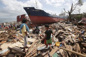
As the Philippines assesses the havoc caused by Typhoon Haiyan, which according to some reports has killed as many as 10,000 people, speculation is heating up as to whether the disaster might be a manifestation of climate change. Speaking today on the first day of United Nations climate talks in Warsaw, the head of the Philippines delegation, Yeb Sano, said that he will stop eating until negotiators make "meaningful" progress.

But can the devastating storm be linked to the changing global climate? Nature wades into the evidence.

Was Haiyan the strongest storm ever measured?

Apparently, yes. With sustained wind speeds of more than 310 kilometres per hour, Haiyan was the most powerful tropical cyclone to make landfall in recorded history. The previous record was held by Hurricane Camille, which hit Mississippi in 1969 with wind speeds of just over 300 kilometres per hour.

It is the third time that disaster has struck the Philippines in less than 12 months. In August, Typhoon Trami caused massive flooding on the island of Luzon. And in December 2012, Typhoon Bopha killed up to 2,000 people and caused some US$1.7 billion in damage on the island of Mindanao. Haiyan could easily surpass that figure: its total economic impact could reach US$14 billion, according to a report by a senior insurance analyst at Bloomberg Industries, a data company in New York.

Haiyan's death toll might have been much bigger had so many people in the Philippines not heeded storm warnings and fled at-risk areas.

What’s the difference between a cyclone, a typhoon and a hurricane?

They are just different names for the same type of extreme weather phenomenon occurring in different parts of the world. These storms are called hurricanes in the Atlantic and northeastern Pacific oceans, typhoons in the northwestern Pacific and cyclones in the south Pacific and Indian Ocean.

Are such storms getting worse in a warming world?

This is the million-dollar question, but there is not yet a scientific consensus on how to answer it.

Storms receive their energy from the ocean, so it would seem logical that they would get stronger, and perhaps also more frequent, as the upper layers of tropical oceans get warmer. The potential intensity of tropical storms does increase with warmer sea surface temperatures. However, the effect of warming seas could be counteracted by the apparent increase in the strength of shearing winds — winds blowing in different directions and varying in strength at different altitudes. Shearing winds tend to hinder the formation of storms, or tear them apart before they can reach extreme strength.

On balance, many climate researchers think that it is plausible that tropical-storm activity will rise as the planet warms. There is some evidence 1 that storm intensity has increased over the last three decades, but reliable data are limited to the north Atlantic, where observations are most abundant. In other places, the evidence is not yet conclusive 2 .

The Intergovernmental Panel on Climate Change (IPCC) in its latest report cautiously summarizes the current state of knowledge:

“Time series of cyclone indices such as power dissipation, an aggregate compound of tropical cyclone frequency, duration, and intensity that measures total wind energy by tropical cyclones, show upward trends in the North Atlantic and weaker upward trends in the western North Pacific since the late 1970s, but interpretation of longer-term trends is again constrained by data quality concerns.”

What are the models saying?

Global climate models are too coarse to resolve relatively small-scale atmospheric disturbances such as tropical storms — despite how prominently these phenomena feature on weather maps. Scientists therefore need to infer the effect of global warming on storm activity from general patterns of atmospheric circulation.

For example, hurricane researcher Kerry Emanuel of the Massachusetts Institute of Technology in Cambridge has used 3 a technique to simulate large numbers of tropical cyclones in climate models. When applied to scenarios of historical and future climate described by six state-of-the-art climate models, his method predicted that both the frequency and intensity of tropical cyclones will increase during the twenty-first century in all tropical ocean regions, except the southwestern Pacific. Emanuel’s study was published too late for inclusion in the latest IPCC report.

Elsner, J. B., Kossin, J. P. & Jagger, T. H. Nature 455 , 92–95 (2008).

Article   ADS   CAS   Google Scholar  

Coumou, D. & Rahmstorf, S. Nature Clim. Change 2 , 491–496 (2012).

Article   ADS   Google Scholar  

Emanuel, K. A. Proc. Natl. Acad. Sci. USA 110 , 12219-12224 (2013).

Download references

You can also search for this author in PubMed   Google Scholar

Related links

Related links in nature research.

IPCC: Despite hiatus, climate change here to stay 2013-Sep-27

Hurricane Sandy spins up climate discussion 2012-Oct-30

Climate panel says prepare for weird weather 2011-Nov-18

Climate and weather: Extreme measures 2011-Sep-07

Most powerful hurricanes on the rise 2010-Jan-21

Nature special: Outlook for Earth

Related external links

NOAA: Hurricanes, cyclones and typhoons

Rights and permissions

Reprints and permissions

About this article

Cite this article.

Schiermeier, Q. Did climate change cause Typhoon Haiyan?. Nature (2013). https://doi.org/10.1038/nature.2013.14139

Download citation

Published : 11 November 2013

DOI : https://doi.org/10.1038/nature.2013.14139

Share this article

Anyone you share the following link with will be able to read this content:

Sorry, a shareable link is not currently available for this article.

Provided by the Springer Nature SharedIt content-sharing initiative

This article is cited by

New insights into the poleward migration of tropical cyclones and its association with hadley circulation.

• Karanam Kishore Kumar

Scientific Reports (2023)

Circular characteristics of the Philippine storm tracks

• Al-Ahmadgaid B. Asaad

Spatial Information Research (2022)

Future projection of maximum potential storm surge height at three major bays in Japan using the maximum potential intensity of a tropical cyclone

• Nobuhito Mori
• Nozomi Ariyoshi
• Junichi Ninomiya

Climatic Change (2021)

Future typhoon and storm surges under different global warming scenarios: case study of typhoon Haiyan (2013)

• Ryota Nakamura
• Tomoya Shibayama
• Takumu Iwamoto

Natural Hazards (2016)

Quick links

• Explore articles by subject
• Guide to authors
• Editorial policies

Sign up for the Nature Briefing newsletter — what matters in science, free to your inbox daily.

Typhoon Haiyan

The Philippines consists of a group of islands in the South China Sea. The country regularly suffers from large typhoons that move in from the south west every year during the tropical storm season. This case study is about Typhoon Haiyan, which is unofficially the fourth most intense tropical cyclone ever observed.

Facts about the Philippines & UK (from CIA Fact book 2014)

BACKGROUND CAUSES

The Philippines sits in an area of seasonally warm ocean water (sea temperatures over 27°C) and has enough Coriolis Force to create rotating winds over the ocean's surface. Sea-level rise is happening globally but is particularly affecting the Philippines. It is caused by global warming and has gone up by about 20cm since 1900. These sea level rises create larger storm surges. Use of groundwater has caused parts of the country to sink. The worst affected city, Tacloban, is at the end of a bay that funnelled water from the storm surge.

NASA image of Typhoon Haiyan By NASA, LAADS Web

Timeline of development; • 2nd November 2013 – Typhoon Haiyan starts as an area of low pressure several hundred kilometers east-southeast of Pohnpei in the Federated States of Micronesia. • 3rd November – moves west and develops into a tropical depression • 4th November - Haiyan becomes a tropical storm • 5th November -  the system began a period of rapid intensification that brought it to typhoon intensity. • 7th November  - Typhoon Haiyan made landfall in  Guiuan, Eastern Samar • 10th to 11th of November - Haiyan reaches Vietnam and weakens in intensity Impacts Quick facts according to the Disasters and Emergency Committee of the UK • Typhoon Haiyan - known locally as Yolanda - hit eastern Samar Island at 8.40pm GMT on 7 November 2013 (4.40am 8th November local time). • It caused a storm surge – a wall of water – that was 25 feet high in some areas, including in the town of Tacloban. • Over 14 million people were affected across 46 provinces. • The city of Tacloban, home to more than 220,000 people, suffered more loss of life than any other area of the Philippines. • Five million people saw their homes severely damaged or destroyed (550,000 houses destroyed and an additional 580,000 houses were severely damaged).

Devastation in Tacloban By Trocaire from Ireland (DSC_0749)

Typhoon Haiyan is one of the most devastating storms of recent history. It killed approximately 7400 people (6,340 confirmed, 1,061 missing) and affected 9 million people. Immediately after the storm the Philippines faced a humanitarian crisis after the Visayas Islands in the central part of the country had 1.9 million homeless and more than 6,000,000 displaced. The economy was affected, with estimated losses at $2.9billion with much of this in agriculture.  The major rice and sugar producing areas for the Philippines were destroyed. A total of 131,611 tons of rice was lost (Food and Agriculture Organisation (FAO)), together with much of the coconut crop which is nearly half the Philippines agricultural exports (the country is the world’s biggest producer of coconut oil).  5.9 million Workers lost income sources according to USAID. Tacloban airport terminal building was also completely destroyed by a 5m storm surge. The United Nations feared the possibility of the spread of disease is high due to the lack of food, water, shelter, and medication. In addition, casualties were reported as a result of the lack of aid in affected areas.  Socially people were affected; they became refugees in lass affected areas and migrated there.  Also, fishing communities were affected with the storm destroying boats and associated equipment. The natural environment was also affected, with loss of forests, trees and widespread flooding. Local ecosystems were also affected by sewage leaking from overwhelmed sewage systems and oil leaks. A lack of sanitation in days following the event also leads to a higher level of pollution.

Management & responses The government was criticised for its slow response to this event. However, the Philippines formally declared "A State of National Calamity" and asked for international help; one day after the Haiyan hit the country.  A week after the typhoon had struck President Benigno Aquino was under growing pressure to speed up the distribution of networks or food, water and medicine to desperate survivors and to get paralysed local governments functioning. However, the storm damaged infrastructure making response difficult.  For example, the Tacloban city government was decimated, with just 70 workers in the immediate days after the disaster compared to 2,500 normally. Many were killed, injured, lost family or were simply too traumatised to work.

By December, water tanks had been installed by charities like Oxfam but not in all areas.  6 Months later, many people still had limited access to shelter and water.  NGOs like the International Red cross were trying to provide adequate settlements, fresh water access and access to jobs/livelihood. The Philippines authorities have invested in disaster risk reduction (DRR) and climate change adaptation (CCA). They spent $624m on this in 2011 – two per cent of the national budget and 0.28 per cent of GDP – while at least five per cent of a local authority's revenue is set aside for its Local Disaster Risk Reduction Management Fund

NEXT TOPIC - UK Weather hazards

©2015 Cool Geography

• Copyright Policy
• Privacy & Cookies
• Testimonials
• Feedback & support

Resources you can trust

Take 10: Typhoon Haiyan

Appealing black and white revision strips to help GCSE students learn and recall key facts about the Typhoon Haiyan case study.

The PowerPoint slides present the key information, associating each fact with an icon to make it memorable through the technique of dual coding. Students can then annotate the printable revision strips or use them to test recall.

The Word document includes exam-style questions on the relative importance of environmental impacts and social impacts, and of short-term and long-term responses. The questions and mark scheme were written with the Eduqas B GCSE geography specification in mind, but the rest of the resource is likely to be relevant to all exam boards.

An extract from the revision tips section:

Connect one idea to the next to create a chain of knowledge. For example:

• Typhoon Haiyan occurred in the Philippines, Pacific Ocean. When did it make landfall?
• On 7 November 2013. And how strong was it?
• Category 5, with gusts of up to 235 mph and a landfall windspeed of 195 mph. What impact did it have on agriculture?
• 71,000 hectares of farmland were affected, and $85 million was lost from damage to farms.

Carry on in the same way, making connections …

All reviews

Resources you might like.

We use cookies. Read more about them in our Privacy Policy.

• Accept site cookies
• Reject site cookies
• Search Search
• Login Login
• Publications

Typhoon Haiyan: lessons from the response and how to prepare for the future

• Issue 63 The Typhoon Haiyan response
• 1 Coordinating the response to Typhoon Haiyan
• 2 Typhoon Haiyan: pushing the limits of DRR?
• 3 Assessing early warning efforts for Typhoon Haiyan in Leyte
• 4 Typhoon Haiyan: lessons from the response and how to prepare for the future
• 5 Constructing a culture of accountability: lessons from the Philippines
• 6 Pamati Kita: 'Let's Listen Together'
• 7 Coordination around communicating with disaster-affected communities: insights from Typhoon Haiyan
• 8 Engaging with clusters: empowering and learning from local organisations
• 9 Humanitarian partnerships: reality lags behind the rhetoric
• 10 ‘Recently noticed’ aid actors: MSF’s interaction with a changing humanitarian landscape
• 11 Are cash transfers the 'new normal' in the Philippines? Challenges and opportunities from Typhoon Haiyan
• 12 The private sector: stepping up
• 13 Urban shelter and settlement recovery: a 'menu of options' for households
• 14 Supporting shelter self-recovery: field experience following Typhoon Haiyan

Responding to multiple disasters

Be prepared, anticipate likely needs, mental health needs, a ‘baby boom’, strengthen long-term resilience.

• Twitter Twitter
• Facebook Facebook
• Share on Email Email

T yphoon Haiyan (known locally as Yolanda) made landfall in the Philippines on 8 November 2013. Just over a year on, this article reflects on what the World Health Organisation (WHO) – the co-lead for the health cluster alongside the Philippines Department of Health (DoH) – has learnt, how these lessons have influenced the response over time and what this means for responses to health emergencies in the future. The article is based on internal information from WHO’s own work, though it is hoped that the main findings will also be useful to other agencies.

The first lesson is that national agencies and the international community need to be ready to respond to multiple natural disasters each year in the Philippines. The country is one of the world’s most disaster-prone. Typhoon Haiyan was the third crisis to hit the country in two months, following conflict in Zamboanga and an earthquake in Bohol, which combined displaced 750,000 people. This meant that response services including national and international agencies and the Philippine army were already stretched.

WHO Philippines has been working with the DoH to set up Emergency Operations Centres in vulnerable areas of the country, and to establish a gold, silver and bronze command system The colours signify different levels of control within a hierarchical framework: gold for strategic, silver for tactical and bronze for operational.  to direct disaster responses. The agency has also been restocking and pre-positioning medical supplies and equipment in anticipation of more natural disasters, and is developing toolkits with the DoH for emergency preparedness. These toolkits will provide guidance on procedures and practices to ensure a quick response in the aftermath of an emergency. Both national and local governments are working to ensure that health structures are disaster resilient.

A second lesson is that, in any emergency response, aid agencies need to be prepared for the situation on the ground. Foreign medical teams need to bring enough food, water, shelter, fuel and communications equipment to be self-sufficient, particularly in areas that are physi-cally cut off and where communications are poor or non-existent. They also need to factor into their pre-arrival planning sufficient health supplies and capacity to deal with the health priorities and ground realities in the Philippines. Some teams came ready to treat the injured but had not considered the immediate demand for services for pregnant mothers or the need to replace daily medications. The country has a triple burden of disease: communicable and non-communicable diseases plus the impact of natural disasters on an already stretched health service. The Philippines also has the highest fertility rate in Asia: for some military medical teams accustomed to treating injuries it was a surprise to find they had to dust off their skills at delivering babies too. Some teams needed additional drug supplies from WHO Philippines to treat chronic heart disease and hypertension.

For efficient use of the medical personnel, facilities and medication brought in by foreign medical teams, it is essential to systematise the procedure for their deployment. WHO Philippines instigated a registration and briefing system to make sure foreign teams were prepared before they were deployed to areas needing support. WHO helped the DoH to coordinate over 150 foreign medical teams during the response. They held over 193,000 consultations, performed over 5,000 surgeries and assisted in over 1,200 deliveries.

A third lesson concerns anticipating what the needs will be during different phases of the response. In the first wave, the initial days and weeks are focused on treating the injured, providing equipment to newly disabled people and attending to pregnant women. A second wave of activity involves the prevention of disease outbreaks through the restarting of surveillance activities to track any potential outbreaks and an immunisation campaign across the whole affected area to protect children against measles, rubella and polio. This is coordinated by the national government, but UN agencies and foreign medical teams provide important support on disease surveillance and often participate in the delivery of immunisation campaigns. Measles is circulating constantly in the Philippines, and after a disaster children living in crowded conditions are particularly vulnerable to developing complications and even dying of the disease. In addition to poor living conditions, there can be large-scale migrations in the aftermath of a major disaster, which are likely to have an impact on immunisation needs.

In the first wave of immunisations conducted in the typhoon-affected area, almost 110,000 children were vaccinated against measles, and an expanded catch-up campaign in the National Capital Region in January–February 2014 saw an additional 1.7 million children immunised. In addition, there is an urgent need to get those living with TB and multi-drug resistant TB (MDR-TB) back on treatment to prevent the spread of the disease and increased drug resistance. The typhoon-affected area had an estimated 26,249 TB cases with 356 cases of MDR-TB. By mid-December almost all TB patients were back in treatment services. There is also a need to prevent other communicable diseases such as dengue, which spreads quickly where mosquitos are able to breed among debris.

Disasters such as Typhoon Haiyan magnify the threat from non-communicable diseases (NCDs) because they disrupt access to and delivery of essential interventions, including medicines. This constitutes a third wave of activity. NCDs are among the top killers in the Philippines, accounting for more than 70% of the deaths recorded in the country annually. Within weeks of the typhoon there was a rise in the number of patients requiring treatment for NCDs, and as the months went on the risk of heart attacks and strokes grew significantly due to the stress of the situation combined with long-term health problems. In the first three months after the disaster, 14,000 consultations were reported for hypertension alone. Another 1,770 consultations were reported for diabetes. The need to address NCDs proactively before a natural disaster and to ensure sufficient care in the aftermath was a key lesson from the response to Haiyan. WHO provided additional supplies for NCD treatment to the foreign medical teams that came to assist in the response as many had not anticipated the level of demand.

Within three to four months after a disaster there is a transition from an emergency response to an early recovery phase. Emergency response activities such as supplementary feeding programmes close down and free health care dries up as foreign medical teams leave. This transition can lead to further health challenges that have to be planned for and managed. For example, in many of the typhoon-affected areas malnutrition was already a problem. The concern was that this would be exacerbated when feeding programmes finished. WHO has been promoting breastfeeding of newborns and infants as a way to improve child health, and has trained health workers to treat severe acute malnutrition in particular. Meanwhile, as public water supply systems are restored, they need to be tested for water quality. Results of water quality testing done in priority areas of region 8 revealed the presence of bacteriological contamination in a third of the samples collected. There was a clear need for training and skills enhancement of water safety engineers to ensure safe water supplies. WHO has trained 340 sanitary inspectors on water quality management and distributed test kits to nine provinces and two cities.

In the first few weeks after a disaster it is essential to provide psychosocial first aid, particularly to people who have lost family, homes or livelihoods. However, mental health impacts begin to really show after around six months, when the initial adrenalin rush dies away and morale and energy dip. Responding to mental health needs requires a fourth wave of activity. WHO estimates that, in humanitarian emergencies, the percentage of people suffering from depression or anxiety disorders can double from a baseline of 10% to about 20%, while the percentage of people with severe mental disorders can increase by up to 50%.

Finally, there is typically a ‘baby boom’ following a disaster. More women become pregnant than previously expected, leading to greater demand for prenatal care and for food and vaccines for children following their birth. This puts additional pressure on health services just as many aid agencies are pulling out. This fifth wave of health needs requires a scaling up of services and a longer-term plan to serve the needs of a growing population.

Given these multiple waves of health needs it is important that health teams do not all rush in at once, but that assistance is staggered to make sure that people’s needs are met for months – not just weeks – after the disaster. This is a question of coordination and requires the support of donors and aid agency managers. WHO Philippines was particularly grateful to those teams that held back and took over once the initial rush had subsided and others had pulled out. It is important to recognise the work that was done after the TV cameras had gone. Considerable health needs remain more than a year after the typhoon, with implications for the management and funding of the health aspects of the response given that most funding tends to finish within 12 months. Ultimately, there has to be a sixth wave of activity: the transition from recovery to development, with a multi-year plan in place to ensure the full restoration of health services to all those in the affected areas. This requires investment in health planning, information management and capacity-building at all levels.

A final lesson therefore concerns how to strengthen resilience for the future, particularly given the frequency and severity of natural disasters in the Philippines. We know that the health facilities that best withstood the typhoon were often originally built and supported by the community. It is at the level of communities that this resilience has to be forged. To build resilience at local level requires improving the skills of community health workers. First aid training can help ensure that communities are able to assist the injured before national and international teams have reached them. Resilience also needs to be built into the construction and management of health facilities, and WHO has included building plans, design parameters and guidelines for rebuilding health facilities in two photobooks published by the DoH, entitled Rising Anew: Health at the Heart of Healing . These health facilities require a predictable supply of clean water and electricity – services that are sadly lacking even in areas not hit by the typhoon. To improve this situation, local officials need to understand where these services are absent and take charge of rectifying this. WHO Philippines has worked hard with the DoH to map the status of health infrastructure and health services. This process is ongoing and will guide recovery operations.

The Philippines faces multiple natural disasters each year, and to respond to them we need to have the right emergency services and systems in place. The structure created to deal with disasters has to be able to handle multiple waves of health needs over months and, in the case of a disaster on the scale of Haiyan, for years after the event. This requires investment in health planning, information management and capacity-building at all levels. WHO Philippines continues to work with the national government and international partners to ensure the full restoration of health services to all those in typhoon-affected areas.

Dr Julie Hall MBE is the WHO Representative to the Philippines.

Comments are available for logged in members only.

Issue 63 Contents

Environmental and Disaster Displacement Policy pp 129–158 Cite as

Typhoon Haiyan: Context, Actors and Response

• Silvana Lakeman 2  
• First Online: 22 October 2021

195 Accesses

This chapter provides an overview of how key actors prepared and reacted to Typhoon Haiyan, and defines key issues surrounding the disaster. Entities considered include the government of the Philippines, the international humanitarian response (of which the United Nations High Commissioner for Refugees [UNHCR] and the International Organization for Migration [IOM] were part) and, finally, affected communities. This chapter introduces, then provides a basic level of context to, the disaster itself and provides a backdrop against which to sufficiently consider and situate specific priorities of the UNHCR and IOM in response to Typhoon Haiyan.

This is a preview of subscription content, log in via an institution .

Buying options

• Available as PDF
• Read on any device
• Instant download
• Own it forever
• Available as EPUB and PDF
• Compact, lightweight edition
• Dispatched in 3 to 5 business days
• Free shipping worldwide - see info
• Durable hardcover edition

Tax calculation will be finalised at checkout

Purchases are for personal use only

Aseo, E. (2014): “Two Months After Yolanda: Lessons from the Bunkhouse Controversy” Asia Foundation. Available at: https://asiafoundation.org/2014/01/15/two-months-after-yolanda-lessons-from-the-bunkhouse-controversy/ , accessed 22 July 2019.

BBC News (2013): “Deadly Philippine quake hits Bohol and Cebu” BBC. Available at: https://www.bbc.com/news/world-asia-24530042 , accessed 20 June 2019.

Biquet, Jean-Marc (2014): “Haiti: Between Emergency and Reconstruction, An inadequate response” International Development Policy/Revue International de Politique de Developpement, 4(3). Available at: https://doi.org/10.4000/poldev.1600 , accessed 26 July 2019.

Brown, Alesh (2015): “Are cash transfers the new normal in the Philippines? Challenges and opportunities from Typhoon Haiyan” Humanitarian Practice Network. Available at: https://odihpn.org/magazine/are-cash-transfers-the-%C2%91new-normal%C2%92-in-the-philippines-challenges-and-opportunities-from-typhoon-haiyan/ , accessed 26 July 2019.

Bueza, Michael (2014): “The role of LGUs, local councils during disasters” Rappler. Available at: https://r3.rappler.com/newsbreak/44026-role-lgu-local-councils-disasters , accessed 19 July 2019.

Carden, David and Clements, Ashley Jonathan (2015): “Coordinating the response to Typhoon Haiyan” Humanitarian Practice Network. Avail-able at: https://odihpn.org/magazine/coordinating-the-response-to-typhoon-haiyan/ , accessed 19 July 2019.

CCCM Philippines (2013): “Typhoon Haiyan/Yolanda Camp Coordination and Camp Management (CCCM) Draft Strategy” CCCM Philippines. Available at: https://cccmphilippines.iom.int/strategy , accessed 29 March 2019.

CCCM Philippines (2019): “DTM” CCCM Philippines. Available at: https://cccmphilippines.iom.int/dtm-main , accessed 29 July 2019.

Cesar I. Trajano, Julius (2016): “Building Resilience from Within: Enhancing Humanitarian Civil-Military Coordination in Post-Haiyan Philippines, NTS Report No. 6” S. Rajaratnam School of International Studies. Available at: https://www.rsis.edu.sg/rsis-publication/nts/building-resilience-from-within-enhancing-humanitarian-civil-military-coordination-in-post-haiyan-philippines/#.XTV90OgzZPY , accessed 20 July 2019.

Chandra Ratha, Keshab and Kumar Mahapatra, Sushanta (2014): “Climate Change and Natural Disasters: Responding to the Philippines’ Hai-yan Tragedy” Quaderni – Working Paper DSE No. 940. Available at: https://papers.ssrn.com/sol3/papers.cfm?abstract_id=2430689 , accessed 19 July 2019.

Ching, Paola Katrina., de los Reyes, Vikki Carr., Sucaldito, Ma Nemia and Tayag, Enrique (2015): “An assessment of disaster-related mortality post-Haiyan in Tacloban City” Western Pacific Surveillance and Response Journal, 6(1): 34–38.

Article   Google Scholar  

Commission on Human Rights, Republic of the Philippines (2018): “A disaster approach to displacement: IDPs in the Philippines” chr.gov.ph . Available at: http:// chr.gov.ph /a-disaster-approach-to-displacement-idps-in-the-philippines/, accessed 18 March 2019.

de Leon, E. G., & Pittock, J. (2017): “Integrating climate change adaptation and climate-related disaster risk-reduction policy in developing countries: A case study in the Philippines” Climate and Development, 9(5): 471–478.

Department of Environment and Natural Resources (2019): “DENR delineates 20 and 40 metres easement of coast lines affected by typhoon Yolanda” gov.ph. Available at: http://r8.denr.gov.ph/index.php/86-region-news-items/320-denr-delineates-20-and-40-meters-easement-of-coast-lines-affected-by-typhoon-yolanda/ , accessed 22 July 2019.

Dy, Philip and Stephens, Tori (2016): “The Typhoon Haiyan Response: Strengthening Coordination among Philippine Government, Civil Society, and International Actors” PCL Discussion Paper Series, Harvard Kennedy School Program on Crisis Leadership. Available at: https://www.hks.harvard.edu/sites/default/files/centers/research-initiatives/crisisleadership/files/Dy_and_Stephens.pdf , accessed 2 December 2019.

Escandor, Alaysa (2016): “3 years after Typhoon Haiyan, data reveals lessons in funding and rehabilitation” Devex. Available at: https://www.devex.com/news/3-years-after-typhoon-haiyan-data-reveals-lessons-in-funding-and-rehabilitation-88993 , accessed 26 July 2019.

Esteban, Miguel., Valenzuela, Ven Paolo., Yi Yun, Nam., Mikami, Takahito., Shibayama, Tomoya., Matsumaru, Ryo., Takagi, Hiroshi., Danh Thao, Nguyen., de Leon, Mario., Oyama, Takahiro., & Nakamura, Ryota (2015): “Typhoon Haiyan 2013 Evacuation Preparations and Awareness” International Journal of Sustainable Future for Human Security, 3(1): 37–45.

Field, Jessica (2017): “What is appropriate and relevant assistance after a disaster? Accounting for culture(s) in the response to Typhoon Hai-yan/Yolanda” International Journal of Disaster Risk Reduction, 22: 335–344.

Global Animal Network (2019): “Typhoon Haiyan, an example of effective response, preparedness and resilience” Global Animal Network. Available at: https://www.globalanimalnetwork.org/typhoon-haiyan-example-effective-response-preparedness-and-resilience , accessed 19 July 2019.

GMA News (2013): “SONA: Tacloban City Mayor Alfred Romualdez, naglabas ng hinanakit kanina sa hearing sa Senado” [Video, Youtube.com ]. Available at: https://www.youtube.com/watch?v=ryXnGhkKOl8 , accessed 1 May 2019.

Government of the Philippines (2013): “Veto Message of President Aquino on Senate Bill No. 3317 and House Bill No. 5627” gov.ph. Available at: https://www.officialgazette.gov.ph/2013/05/24/veto-message-of-president-aquino-on-senate-bill-no-3317-and-house-bill-no-5627/ , accessed 20 February 2019.

Government of the Philippines (2014): “Resolution directing the committees on aquaculture and fisheries resources and public works and highways to conduct a joint inquiry, in aid of legislation, on the impact of the ‘no-build zone, no-dwell-zone policy’ being implemented in coastal areas affected by super typhoon Yolanda” gov.ph. Avail-able at: http://www.congress.gov.ph/legisdocs/basic_16/HR00947.pdf , accessed 22 July 2019.

Government of the Philippines (2019): “Overseas Filipinos’ (OF) Remittances” gov.ph. Available at: http://www.bsp.gov.ph/statistics/keystat/ofw.htm , accessed 17 July 2019.

Hanley, Teresa., Binas, Rusty., Murray, Julian and Tribunalo, Baltz (2014): “IASC Inter Agency Humanitarian Evaluation of the Typhoon Haiyan Response, Prepared on behalf of the Inter Agency Humanitarian Evaluation Steering Group, October 2014” UN OCHA. Available at: https://www.unhcr.org/research/evalreports/583305867/iasc-inter-agency-humanitarian-evaluation-typhoon-haiyan-response.html , accessed 18 March 2019.

Hartmann, Christoph., Rhoades, Amy and Santo, Jerby (2014): “Starting the Conversation: Information, Feedback and Accountability Through Communications with Communities in Post-Typhoon Philippines” IOM. Available at: http://www.cdacnetwork.org/contentAsset/raw-data/3930b1cb-c03a-4a37-8e2f-39e20bc810d7/attachedFile , accessed 3 July 2019.

Howe, Brendan and Bang, Geehyun (2017): “Nargis and Haiyan: The Politics of Natural Disaster Management in Myanmar and the Philippines” Asian Studies Review, 41(1): 58–78.

Humanitarian Practice Network (2015): “Humanitarian Exchange, Special feature, The Typhoon Haiyan response, Number 63” Humanitarian Practice Network. Available at: https://odihpn.org/wp-content/uploads/2015/01/HE_63_new_web2_.pdf , accessed 23 July 2019.

IASC (2012a): “Reference Module for Cluster Coordination at the Country Level” IASC. Available at: https://www.refworld.org/pdfid/512dedd22.pdf , accessed 23 July 2019.

IASC (2012b): “Inter Agency Standing Committee Transformative Agenda Reference Document. 2. Humanitarian System-Wide Emergency Activation: Definition and procedures PR/1204/4078/7” IASC. Available at: https://www.refworld.org/pdfid/512deb632.pdf , accessed 22 July 2019.

IASC (2019a): “IASC Inter Agency Standing Committee” IASC. Available at: https://interagencystandingcommittee.org/ , accessed 25 February 2019.

IASC (2019b): “IASC Transformative Agenda, Timeline: Scaling-up a Response with the IASC Scale-Up Protocols” IASC. Available at: https://interagencystandingcommittee.org/iasc-transformative-agenda , accessed 2 April 2019.

IFRC (2017): “Emergency appeal final report, Philippines: Typhoon Haiyan” International Federation of Red Cross and Red Crescent Societies. Available at: https://reliefweb.int/sites/reliefweb.int/files/resources/MDRPH014FR.pdf , accessed 24 July 2019.

Inter-cluster Coordination Group for the Humanitarian Country Team (2014): “2014 Final Periodic Monitoring Report Typhoon Haiyan (Yolanda)” Humanitarian Response. Available at: https://www.humanitarianresponse.info/sites/www.humanitarianres-ponse.info/files/documents/files/20141022%20PHI%20Haiyan%20PMR3%20final.pdf , accessed 4 June 2019.

International Organization for Migration (2013a): “In the Philippines, a relief effort of giant proportions and fiendishly complicated logistics is under way” IOM. Available at: https://www.iom.int/news/philippines-relief-effort-giant-proportions-and-fiendishly-complicated-logistics-under-way , accessed 2 January 2019.

International Organization for Migration (2013b): “Typhoon Haiyan: IOM Philippines Situation Report, 18 November 2013” IOM. Available at: https://www.iom.int/files/live/sites/iom/files/Country/docs/IOM-Typhoon-Haiyan-SitRep-20131118.pdf , accessed 2 January 2019.

International Organization for Migration (2014): “Typhoon Haiyan: Portraits of Recovery” IOM Mission in the Philippines. Available at: https://publications.iom.int/books/typhoon-haiyan-portraits-recovery , accessed 19 March 2019.

International Organization for Migration (2019): “IOM Philippines” IOM. Available at: https://www.iom.int/countries/philippines , accessed 21 August 2019.

IRIN (2014): “‘No-build zones’ confusion delays resettlement of Haiyan survivors” IRIN News. Available at: http://www.irinnews.org/report/100368/%E2%80%9Cno-build-zones%E2%80%9D-confusion-delays-resettlement-haiyan-survivors , accessed 18 March 2019.

Kim P. Yee, Dalika (2018): “Constructing reconstruction, territorializing risk: Imposing ‘no-build zones’ in post-disaster reconstruction in Tacloban City, Philippines” Critical Asian Studies, 50(1): 103–121.

Lagmay, Alfredo Mahar Francisco., Agaton, Rojelee P., Bahala, Mark Allen C., Briones, Jo Brianne Louise T., Cabacaba, Krichi May C., Caro, Carl Vincent C., Dasallas, Leo L., Gonzalo, Lia Anne L., Ladiero, Christine N., Lapidez, John Philip., Mungcal, Maria Theresa Francia., Puno, Jose Victor R., Ramos, Michael Marie Angelo C., Santiago, Joy., Suarez, John Kenneth and Tablazon, Judd P. (2015): “Devastating storm surges of Typhoon Haiyan” International Journal of Disaster Risk Reduction, 11: 1–12.

Lofts, Katherine and Kenny, Alex (2012): “Mainstreaming climate resilience into government: The Philippines’ Climate Change Act” Climate and Development Knowledge Network. Available at: https://cdkn.org/wp-content/uploads/2012/07/Philippines-InsideStory_6pp_WEB3.pdf , accessed 19 July 2019.

Mas, E., Bricker, J., Kure, S., Yi, C., Suppasri, A., & Koshimura, S. (2015): “Field Survey report and satellite image interpretation of the 2013 Super Typhoon Haiyan in the Philippines” Natural Hazards and Earth System Sciences, 15: 805–816.

McElroy, Andy (2013): “Evacuation saves whole island from Typhoon Haiyan” UNISDR. Available at: https://www.unisdr.org/archive/35524 , accessed 22 July 2019.

Morden, Johanna (2014): “Typhoon Haiyan: Indigenous people seek to break cycle of displacement” UNHCR. Available at: https://www.unhcr.org/news/latest/2014/2/52f0c8e36/typhoon-haiyan-indigenous-people-seek-break-cycle-displacement.html , accessed 31 August 2018.

Moretti, Sebastien (2020): “Between refugee protection and migration management: the quest for coordination between UNHCR and IOM in the Asia-Pacific region” Third World Quarterly, 42(1): 34-51.

NDRRMC (2019): “National Disaster Risk Reduction and Management Council” NDRRMC Operation Center. Available at: http://www.ndrrmc.gov.ph/ , accessed 25 February 2019.

Nobuhito, Mori., Kato, Masaya., Kim, Sooyoul., Mase, Hajime., Shibutani, Yoko., Takemi, Tetsuya., Tsuboki, Kazuhisa and Yasuda, Tomohiro (2014): “Local amplification of storm surge by Super Typhoon Haiyan in Leyte Gulf” Geophysical Research Letters, 41(14): 5106-5113.

Norwegian Refugee Council (2019): “Women and Youth Speak: Faces of Disaster Displacement” [Conference Event]. Global Platform for Disaster Risk Reduction, 15 May 2019, Geneva, Switzerland. Available at: https://www.unisdr.org/conference/2019/globalplatform/programme/side-events/view?id=928 , accessed 15 May 2019.

Ong, Jonathan C., Flores, Jaime M and Combinido, Pamela (2015): “Obliged to Be Grateful: How Local Communities Experienced Humanitarian Actors in the Haiyan Response” PLAN International. Available at: https://plan-international.org/publications/obliged-be-grateful , accessed 26 February 2019.

OXFAM (2014): “In the Shadow of the Storm, OXFAM Briefing Paper” OXFAM. Available at: https://oxfamilibrary.openrepository.com/bitstream/handle/10546/333586/bp-shadow-storm-haiyan-recovery-philippines-061114-en.pdf?sequence=1 , accessed 22 July 2019.

Palatino, Wong (2015): “Philippines Must Protect Internally Displaced Persons, Warns UN Expert” The Diplomat. Available at: https://thediplomat.com/2015/08/philippines-must-protect-internally-displaced-persons-warns-un-expert/ , accessed 18 March 2019.

Paragas, Gerald., Rodil, Amillah and Pelingon, Lysandre (2016): “Tacloban after Haiyan: Working together towards recovery” IIED. Available at: https://pubs.iied.org/10798IIED/ , accessed 17 July 2019.

Philippines Humanitarian Response (2013): “Philippines: Bohol Earthquake Action Plan October 2013” Reliefweb. Available at: https://reliefweb.int/sites/reliefweb.int/files/resources/Bohol%20Earthquake%20Action%20Plan%20FINAL_0.pdf , accessed 14 April 2019.

Protection Cluster Philippines (2015): “Haiyan (Yolanda)” Protection Cluster Philippines. Available at: http://www.protectionclusterphilippines.org/?page_id=41 , accessed 29 March 2019.

Rappler (2013): “Aquino vetoes bill on internally displaced persons” Rappler. Available at: https://www.rappler.com/nation/30200-aquino-vetoes-internally-displaced-persons-bill , accessed 3 November 2019.

Recovery Assistance on Yolanda (2015): “DILG releases ‘Build Back Better’ Operations Manual to strengthen post disaster recovery efforts” gov.ph. Available at: http://ray.dilg.gov.ph/news/765/DILG+releases+%E2%80%98Build+Back+Better%E2%80%99+Operations+Manual+to+strengthen+post-disaster+recovery+efforts/ , accessed 21 March 2019.

Relief Web (2013): “CCCM Hubs Humanitarian Response to Typhoon Haiyan (as of 15 November 2013)” IOM. Available at: https://reliefweb.int/map/philippines/cccm-hubs-humanitarian-response-typhoon-haiyan-15-november-2013 , accessed 29 March 2019.

Santiago, J Sedrey S., Manuela Jr, Wilfred S., Tan, Marion Lara L., Sanez, Siegfried Kiel and Tong, Aldo Zelig U (2016): “Of timelines and timeliness: Lessons from Typhoon Haiyan in early disaster response” Disasters, 40(4): 644–666

Santos, Reynaldo (2013): “Timeline: Super Typhoon Yolanda (Haiyan)” Rappler. Available at: https://www.rappler.com/nation/43316-timeline-super-typhoon-yolanda , accessed 19 February 2019.

Sidel, John T (2014): “The Philippines in 2013: Disappointment, Disgrace, Disaster” Asia Survey, 54(1): 64–70

Smith, Gabrielle (2015): “Cash Coordination in the Philippines: A Review of Lessons Learned During the Response to Super Typhoon Haiyan” OXFAM. Available at: https://oxfamilibrary.openrepository.com/bitstream/handle/10546/557230/er-cash-coordination-philippines-010315-en.pdf?sequence=1&isAllowed=y , accessed 22 July 2019.

Tito Santos, Carlos., Toda, Luigi., Ravi Orduna, Justine., Duarte Santos, Filipe and Ferrao, Joao (2016): “The impacts of Typhoon Haiyan in the Philippines: Implications to land use planning” Climate, Disaster and Development Journal, 1(1): 57–66

Google Scholar  

Tran, Mark (2014): “Typhoon Haiyan disaster response: How the relief effort worked” The Guardian. Available at: https://www.theguardian.com/global-development/poverty-matters/2014/feb/07/typhoon-haiyan-disaster-response-philippines-relief-effort , accessed 2 December 2019.

Tupaz, Voltaire (2014): “Champions for disaster responders: Anyone?” Rappler. Available at: https://www.rappler.com/move-ph/issues/disasters/76354-champions-disaster-responders-anyone , accessed 19 July 2019.

UN High Commissioner for Refugees (2019): “Protection Cluster” UNHCR.Available at: https://www.unhcr.org/ph/protection-cluster , accessed 1 September 2018.

UN OCHA (2013a): “MIRA: Multi-Cluster/Sector Initial Rapid Assessment Philippines Typhoon Haiyan, November 2013” Reliefweb. Available at: https://reliefweb.int/report/philippines/mira-multi-clustersector-initial-rapid-assessment-philippines-typhoon-haiyan , accessed 14 March 2019.

UN OCHA (2013b): “Typhoon Haiyan Strategic Response Plan Factsheet” Reliefweb. Available at: https://reliefweb.int/report/philippines/typhoon-haiyan-strategic-response-plan-factsheet , accessed 22 March 2019.

UNHCR Philippines (2019): “UNHCR in the Philippines” UNHCR. Available at: https://www.unhcr.org/ph/unhcr-in-the-philippines , accessed 29 March 2019.

United Methodist Committee on Relief (2013): “Phases of Disaster Recovery: Emergency Response for the Long Term” Reliefweb. Available at: https://reliefweb.int/report/world/phases-disaster-recovery-emergency-response-long-term , accessed 23 June 2019.

United Nations Human Rights Office of the High Commissioner (2015): “Statement of the United Nations Special Rapporteur on the human rights of internally displaced persons, Chaloka Beyani, on the conclusion of his official visit to the Philippines, 21 to 31 July 2015” OHCHR. Available at: https://ohchr.org/EN/newsEvents/Pages/DisplayNews.aspx?NewsID=16280&LangID=E , accessed 18 March 2019.

UNOCHA (2019): “Coordination” UNOCHA. Available at: https://www.unocha.org/philippines/coordination , accessed 17 June 2019.

van den Homberg, Marc., Meesters, Kenny and Van de Walle, Bartel (2014): “Coordination and Information Management in the Haiyan Response: Observations from the field” Procedia Engineering, 78: 49–51

Walch, Colin (2017): “Typhoon Haiyan: Pushing the limits of resilience? The effect of land inequality on resilience and disaster risk reduction policies in the Philippines” Critical Asian Studies, 50(1): 122–135

World Vision (2019): “2013 Typhoon Haiyan: Facts, FAQs, and how to help” World Vision. Available at: https://www.worldvision.org/disaster-relief-news-stories/typhoon-haiyan-facts , accessed 16 April 2019.

Yamada, Seiji and Absalon, Galat (2014): “Typhoon Yolanda/Haiyan and Climate Justice” Disaster Medicine and Public Health Preparedness, 8(5): 432–435.

Download references

Author information

Authors and affiliations.

Bremen International Graduate School of Social Sciences, University of Bremen, Bremen, Germany

Silvana Lakeman

You can also search for this author in PubMed   Google Scholar

Rights and permissions

Reprints and permissions

Copyright information

© 2022 The Author(s), under exclusive license to Springer Nature Switzerland AG

About this chapter

Cite this chapter.

Lakeman, S. (2022). Typhoon Haiyan: Context, Actors and Response. In: Environmental and Disaster Displacement Policy. Palgrave Macmillan, Cham. https://doi.org/10.1007/978-3-030-84539-1_4

Download citation

DOI : https://doi.org/10.1007/978-3-030-84539-1_4

Published : 22 October 2021

Publisher Name : Palgrave Macmillan, Cham

Print ISBN : 978-3-030-84538-4

Online ISBN : 978-3-030-84539-1

eBook Packages : Political Science and International Studies Political Science and International Studies (R0)

Share this chapter

Anyone you share the following link with will be able to read this content:

Sorry, a shareable link is not currently available for this article.

Provided by the Springer Nature SharedIt content-sharing initiative

• Publish with us

Policies and ethics

• Find a journal
• Track your research

Emergency Management Service - Mapping

Search form

You are here.

• What is Copernicus?
• What is CEMS - Mapping?
• Link to Early Warning Systems

• 2023-11-30 | [EMSN182] Ground deformation monitoring in Brava Island, Cape Verde
• 2023-09-01 | [EMSN171] Flood simulation in Bremen, Germany
• 2023-07-21 | [EMSN157] Region-wide economic asset mapping for Andalusia, Spain.
• 2023-08-24 | [EMSN166] Post-wildfire damage assessment in East Macedonia, Greece
• 2024-02-04 | [EMSR715] Wildfire in Valparaiso region, Chile
• 2023-11-23 | [EMSN183] Forest fire impact assessment in Sierra de Los Guajares, Spain

Damage assessment exploiting remote sensing imagery: Review of the typhoon Haiyan case study

EMS - MAPPING

• Who can use the service
• How to use the service
• Portfolio: Rapid Mapping
• Portfolio: Risk and Recovery
• Quality control

RAPID MAPPING

• List of Activations
• Online Manual

RISK AND RECOVERY

• Map of Activations
• GeoRSS Feed
• Map of Activations of Other Organizations
• Meetings, Workshops
• Citation Guidelines
• Press Mentions
• Calls for Tender

2013 State of the Climate: Record-breaking Super Typhoon Haiyan

Debris lines the streets of Tacloban, Leyte Island. Photo by Trocaire, via Wikimedia .

In the early hours of November 8, 2013, Super Typhoon Haiyan raged into the southern Philippines. The Category 5 storm struck the Visayas region with devastating winds and towering waves. The storm struck with such force that even government-designated storm shelters were swept away. Haiyan, locally known as “Yolanda,” was the deadliest typhoon in the country’s modern record. The storm affected more than 16 million people and left 4 million homeless. In its most recent update from April 2014, the Philippine government confirmed 6,300 dead and more than 1,000 still missing.

Haiyan slammed into the east coast of Samar and Leyte with what may have been the highest recorded wind speed for a tropical cyclone at landfall. The Joint Typhoon Warning Center assigned Haiyan’s one-minute sustained winds at 170 knots (196 mph) when the storm first made landfall in eastern Samar. Although this estimate is still awaiting official validation, it would make Haiyan the strongest tropical cyclone ever recorded at landfall. The previous record of 165 knots (190 mph) is shared by Hurricanes Camille (1969) and Allen (1980) and Super Typhoon Tip (1979).

Haiyan was unusual not just for its record strength, but for its location: it’s very uncommon for tropical cyclones to form so close to the equator. The storm formed at a very low latitude, south of Pohnpei Island (~ 5° N), before swiftly moving westward through Micronesia. It developed into a super typhoon just east of Palau and caused immense property damage in the Kayangel Atoll. It then continued on a west-northwest track before making landfall in the Philippines.

Tracks for the thousands of Eastern Hemisphere tropical cyclones documented in the International Best Track Archive for Climate Stewardship database for 1842-2012. Rarely do storms form within ~5° of the equator. Map by Dan Pisut, NOAA Environmental Visualization Lab.

Haiyan’s intense formation was even more notable because a similarly uncommon low-latitude storm—the deadly Super Typhoon Bopha—hit both Palau and the southern Philippines less than a year earlier in December 2012.

Samar and Leyte Islands suffered the most devastating damage, where the storm surge decimated the coastal city of Tacloban. Tacloban is located in a particularly vulnerable position at the head of San Pedro Bay; much of the city sits a mere five meters above sea level. Early estimates found that the storm surge may have reached a record-high of 7.5 meters (24.6 ft), making Haiyan a contender for the highest storm surge ever observed in the Philippines or East Asia. Eyewitness reports from downtown Tacloban have contributed to even higher surge estimates of 8.5-9.1 meters (27.9 – 29.8 ft). The current surge record of 7.3 meters (23.9 ft) was set in the Philippines in 1897.

Historically high sea levels may have contributed to the storm’s destructive force. Sea level around the central Philippines has risen 200 millimeters (7.9 in) since 1970. Higher sea levels contribute to increased coastal flooding and impact during storm surge events. Fortunately, the peak storm surge at Tacloban occurred at a time of relatively low tide; had the peak surge occurred at high tide, the water level would have been 0.5 meters (1.6 ft) higher.  

Aerial view of damaged homes on Binuluanguan Island, Phillippines. Photo by Keith Morgan, via Wikimedia .

Haiyan actually made five additional landfalls in the Philippines before emerging over the South China Sea, turning northwestward, and striking northern Vietnam as a severe tropical storm on November 10. Months later, the storm’s impact resulted in a massive relief and relocation effort. Ambitious resiliency planning is underway to help mitigate and prepare for similarly destructive typhoons that may strike the region in the future.

M. Lander, C. Guard and S.J. Camargo, 2014: [The Tropics] Sidebar 4.2: Super Typhoon Haiyan [in “State of the Climate in 2013”]. Bull. Amer. Meteor. Soc. , 95 (7), S112-S114.

O. Teves and C. Bodeen (2013, November 11). Haiyan Storm Surges Caught Philippines by Surprise . Associated Press . Accessed June 24, 2014.

L. Buchanan, H. Fairfield, A. Parlapiano, S. Peçanha, T. Wallace, D. Watkins and K. Yourish (2013, November 11) Mapping the destruction of Typhoon Haiyan. New York Times . Accessed June 24, 2014.

Republic of the Philippines National Disaster Risk Reduction and Management Council. Updates re the Effects of Typhoon “Yolanda” (Haiyan), 17 April 2014 . Accessed June 24, 2014.

U.N. Development Program (2014, May). UNDP Supports Typhoon Recovery and Resilience in the Visayas . Accessed June 25, 2014.

B. Dec (2014, June 13). Rebuilding Livelihoods in the Philippines Post-Typhoon Haiyan . White House Initiative on Asian Americans and Pacific Islanders. Accessed June 24, 2014.

We value your feedback

Help us improve our content

Typhoon Haiyan: Four Questions About This Super Storm and Major Humanitarian Disaster

Subscribe to this week in foreign policy, elizabeth ferris elizabeth ferris former brookings expert, research professor, institute for the study of international migration - georgetown university @beth_ferris.

November 12, 2013

Editor’s note: Elizabeth Ferris wrote a follow-up to this post on Typhoon Haiyan and the failure of the Filipino government and the international community to respond immediately to the humanitarian crisis.

The images of coming out of the Philippines are shocking – the scope of the devastation and the depth of the humanitarian crisis left in Typhoon Haiyan’s wake is seemingly immeasurable. As I wait in airport lounges between flights, I am glued to television reports and Twitter posts coming from cities like Tacloban, which was largely flattened by the super storm. While the horrific first images bring tears to my eyes, my Twitter feed mostly reassures me — Oxfam, PACOM, World Vision, UNHCR, USAID and many aid groups are on their way. I receive regular bulletins from the U.N.’s Office for the Coordination of Humanitarian Affairs (OCHA). This is a disaster of enormous proportions, but OCHA is doing what it is supposed to do — coordinating donor contributions, sending regular updates, reporting on the establishment of humanitarian hubs, etc.

As I talk with reporters and try to put this tragedy into perspective, I’m struck by how some in the media see this disaster as a totally new phenomenon. So far, in the aftermath of Typhoon Haiyan — and after years of working on human displacement caused by major natural disasters — I don’t see anything new, although this disaster is certainly much larger than others resulting from the 20 or so cyclones the Philippines experiences every year .

I don’t know how things will turn out in this particular disaster — maybe it will be like the March 2011 earthquake and tsunami in Japan where the initial response was exemplary, but then the meltdown of the Fukushima nuclear reactor demonstrated that the scope of a disaster and the limitations of disaster response can reveal itself over a number of days. Things can always go terribly wrong.

Given that cautionary note, here are four questions to keep in mind as you watch news of the Typhoon Haiyan disaster unfold in the days and weeks ahead:

1. Why do initial government responses appear lacking?

Be wary of initial news reports, especially those of inadequate response by the government of the Philippines. While I’m sure valid reports of government missteps will emerge over time, the Philippine government has invested heavily in disaster preparedness and response. The Philippines has strong civil society organizations, including the Filipino Red Cross, and has practiced, drilled and prepared for disasters for years. I’ve always thought that the Philippines should be given the opportunity to be a leader in teaching other countries about disaster preparedness. In fact, hundreds of thousands of people were evacuated before the cyclone hit. However, there weren’t enough safe areas to accommodate all of the evacuees (remember that the Philippines is made up of thousands of islands). The government should be credited for doing the right thing and evacuating as many people as it could.

2. In some Philippine cities and towns, the images of looting by desperate people look terrible. How widespread is the looting?

Beware of stories about looting in this and other disasters. Looting is always a familiar disaster narrative in news reports. The extent of looting often turns out to be magnified by news coverage and greatly exaggerated after the disaster passes. Hurricane Katrina is a perfect case in point. A few stores sadly were extensively looted — the vast majority of businesses and homes were not.

3. Why does it seem that the poorest are always hit hardest by disasters?

Sadly, poor and marginalized populations always bear the brunt of natural hazards. Even in more stable times, the social safety net supporting these people is often minimal at best. This was true with Hurricane Katrina, true in the 2004 tsunami, true in the hundreds of natural disasters that go unreported or unnoticed each year. It is also true that local groups and communities carry out the bulk of initial response. As you watch the news, look for signs of local Filipino groups — neighbors, churches, local charities — responding quickly to the crisis.

4. Why do responses to disasters always seem late in coming and uncoordinated?

When you don’t know what’s happening, it’s easy to blame the lack of coordination. The truth is that coordination is always difficult when national and local governments are still assessing and communicating need. Lack of coordination is also often difficult for the best of reasons: lots of people and countries want to help but national disaster response capabilities (sometimes due to closed ports and airfields) and international capacities can be limited. Yes, let’s continue to work to improve coordination mechanisms, but let’s not be too quick to point the finger at coordination failures when other factors may be to blame.

Hoping that people appreciate the cautionary notes above, I am heartened as by the outpouring of compassion in response to Typhoon Haiyan. I am proud that USAID, the U.S. military and other branches of the U.S. government are mobilizing a robust response, and I am proud that the United Nations is responding quickly and effectively. I am glad that the media are covering this disaster and hope that Americans and others will respond quickly and generously to the desperate human need. This is a terrible tragedy and the humanitarian needs are great.

We should also keep in mind that, given the reality of climate change, we are likely to see more of these super-disasters in the future. They will be massive and more unpredictable. Disasters like Haiyan are likely to be the new norm. We need to get ready — all of us, Japan, the U.S., the Philippines and hundreds of other countries — as more of these super-disasters are coming our way.

Humanitarian & Disaster Assistance Migrants, Refugees & Internally Displaced Persons

Foreign Policy

Asia & the Pacific

Tarek Ghani, Juan S. Lozano, Anouk Rigterink, Jacob N. Shapiro

March 13, 2024

David G. Victor

December 7, 2023

Rahul Tongia

November 29, 2023

• International
• Schools directory
• Resources Jobs Schools directory News Search

Typhoon Haiyan Case Study Lesson

Subject: Geography

Age range: 14-16

Resource type: Lesson (complete)

Last updated

11 May 2020

• Share through email
• Share through twitter
• Share through linkedin
• Share through facebook
• Share through pinterest

Typhoon Haiyan case study lesson and writing mat/frame resource, corresponding with the AQA GCSE Geography Syllasbus. Fully resourced lesson including a range of activities such as map work, categorising impacts/responses, unpicking an exam answer and an exam style question.

Tes paid licence How can I reuse this?

Your rating is required to reflect your happiness.

It's good to leave some feedback.

Something went wrong, please try again later.

teacherireland

Where is the exam answer? After I purchased this, I can see a mark scheme but the 9 mark question itself is not answered. Where can I get it?

MissGeography26

The question would be answered by the students, which can then be teacher/self or peer assessed using the markscheme.

Empty reply does not make any sense for the end user

Report this resource to let us know if it violates our terms and conditions. Our customer service team will review your report and will be in touch.

Not quite what you were looking for? Search by keyword to find the right resource:

We are sorry Physics & Maths Tutor is slow. There's so many of you visiting at the same time, it's struggling. We are releasing an update later this week.

Physics Revision

Rafael I. ★ 4.9 (12)

University of strathclyde - msc physics.

Patient, friendly and encouraging tutor of physics and maths - broad experience of teaching different levels and ages.

For each of the exam boards below, there are revision notes, factsheets, questions from past exam papers separated by topic and videos.

GCSEs & IGCSEs

A-levels from 2015, international a-levels, uk legacy a-levels, connect with pmt education.

• Revision Courses
• Past Papers
• Solution Banks
• University Admissions
• Numerical Reasoning
• Legal Notices