finite difference method research papers

Finite Difference Method

Ieee account.

• Change Username/Password
• Update Address

Purchase Details

• Payment Options
• Order History
• View Purchased Documents

Profile Information

• Communications Preferences
• Profession and Education
• Technical Interests
• US & Canada: +1 800 678 4333
• Worldwide: +1 732 981 0060
• Contact & Support
• About IEEE Xplore
• Accessibility
• Terms of Use
• Nondiscrimination Policy
• Privacy & Opting Out of Cookies

A not-for-profit organization, IEEE is the world's largest technical professional organization dedicated to advancing technology for the benefit of humanity. © Copyright 2024 IEEE - All rights reserved. Use of this web site signifies your agreement to the terms and conditions.

• Architecture and Design
• Asian and Pacific Studies
• Business and Economics
• Classical and Ancient Near Eastern Studies
• Computer Sciences
• Cultural Studies
• Engineering
• General Interest
• Geosciences
• Industrial Chemistry
• Islamic and Middle Eastern Studies
• Jewish Studies
• Library and Information Science, Book Studies
• Life Sciences
• Linguistics and Semiotics
• Literary Studies
• Materials Sciences
• Mathematics
• Social Sciences
• Sports and Recreation
• Theology and Religion
• Publish your article
• The role of authors
• Promoting your article
• Abstracting & indexing
• Publishing Ethics
• Why publish with De Gruyter
• How to publish with De Gruyter
• Our book series
• Our subject areas
• Your digital product at De Gruyter
• Contribute to our reference works
• Product information
• Tools & resources
• Product Information
• Promotional Materials
• Orders and Inquiries
• FAQ for Library Suppliers and Book Sellers
• Repository Policy
• Free access policy
• Open Access agreements
• Database portals
• For Authors
• Customer service
• People + Culture
• Journal Management
• How to join us
• Working at De Gruyter
• Mission & Vision
• De Gruyter Foundation
• De Gruyter Ebound
• Our Responsibility
• Partner publishers

Your purchase has been completed. Your documents are now available to view.

Numerical solution for two-dimensional partial differential equations using SM’s method

In this research paper, the authors aim to establish a novel algorithm in the finite difference method (FDM). The novel idea is proposed in the mesh generation process, the process to generate random grids. The FDM over a randomly generated grid enables fast convergence and improves the accuracy of the solution for a given problem; it also enhances the quality of precision by minimizing the error. The FDM involves uniform grids, which are commonly used in solving the partial differential equation (PDE) and the fractional partial differential equation. However, it requires a higher number of iterations to reach convergence. In addition, there is still no definite principle for the discretization of the model to generate the mesh. The newly proposed method, which is the SM method, employed randomly generated grids for mesh generation. This method is compared with the uniform grid method to check the validity and potential in minimizing the computational time and error. The comparative study is conducted for the first time by generating meshes of different cell sizes, i.e. , 10 × 10 , 20 × 20 , 30 × 30 , 40 × 40 using MATLAB and ANSYS programs. The two-dimensional PDEs are solved over uniform and random grids. A significant reduction in the computational time is also noticed. Thus, this method is recommended to be used in solving the PDEs.

Abbreviations

two-dimensional

conjugate gradient method

finite difference method

Gauss–Siedel

partial differential equation

Sanaullah Mastoi’s method

1 Introduction

The numerical solution of the partial differential equation (PDE) is mostly solved by the finite difference method (FDM). The FDM is an approximate numerical method to find the approximate solutions for the problems arising in mathematical physics [ 1 ], engineering, and wide-ranging phenomenon, including transient, linear, nonlinear and steady state or nontransient cases [ 2 , 3 , 4 ]. This method is applied to various geometries, distinct boundary conditions and bodies composed of different materials [ 5 ]. FDM applications can easily solve the complex discretization and mathematical modeling computational codes [ 6 ]. Therefore, FDM has been considered to be the critical method for solving practical models [ 7 ]. Many numerical solution techniques [ 8 ] are now available to solve PDEs after high-performance[ 9 ] computing development with extensive storage capability [ 10 , 11 , 12 , 13 , 14 ]. However, the most desirable method for the solution of PDEs is the FDM [ 6 , 15 ].

The heat equation model is an elliptic type PDE [ 16 , 17 ]. The engineering model is commonly solved using the FDM on uniform grids [ 18 ]. However, very few studies have been reported that have applied random step sizes [ 5 , 11 ]. The heat equation theory was developed for modeling how heat diffuses through a given region [ 19 , 20 , 21 ]. The homogeneous heat equation plays a vital role in studying heat conduction and other diffusion processes [ 6 , 22 ].

PDEs can be used to solve various engineering, mathematical, and medical problems involving multiple unknown variables [ 23 , 24 , 25 , 26 ]. The numerical schemes with theoretical analysis focus on the convergence of numerical solution and it is observed that the behavior of randomness was found better during random walk [ 27 , 28 , 29 ]. The various numerical systems are only consistent with limited Fourier steps, spatial steps and the converging steps during the continuous time and solution. The simulation was repeated several times and it was observed that random meshes could reduce the iteration due to their random behavior in cell sizes [ 30 , 31 ].

The numerical solution of PDE using the FDM over uniform meshes has been extensively studied. However, randomly generated grids are also proposed [ 32 , 33 , 34 ]. To the best of the authors’ knowledge, no study is found in the open literature that discusses the validity and potential of randomly generated grids over uniform grids. The solution of fractional PDEs [ 35 , 36 ], Laplace transform, the inverse Laplace transform method through Bernoulli polynomials [ 36 , 37 , 38 ], PDE solutions compared with the domain decomposition method, the θ (theta) method and nonlinear local PDEs [ 7 , 39 ] have previously been carried out using the FDM [ 37 , 40 ]. This study can be extended to the conjugate gradient method (CGM) and GMRES method. The CGM is used for one sample at each iteration [ 41 , 42 , 43 ]. The idea can be proposed on the GMRES method and CGM. The GMRES method is minimizing a step norm of the residual vector over the Krylov subspace. The CGM is used for large-scale data analysis, and the study focuses on the iteration of one sample and the norm of residuals [ 44 , 45 , 46 ].

The geometric representation for the grids (mesh) on the larger domain is discretized in smaller grids. Mesh types such as moving mesh and coupled moving mesh are applied to quasi-linear PDEs for the solution of problems such as magneto-hydrodynamics and the free-surface viscoelastic flow [ 47 , 48 , 49 , 50 , 51 , 52 ]. The mesh generation process needs advancement in engineering models for accuracy and less computational cost [ 53 ]. Additionally, strand meshes have also been used to solve problems involving the flow of multiphase, viscous, and low-speed fluids. However, the mesh generation process is just a past practice. Typically, selecting a suitable mesh generation process for a particular problem becomes difficult, as no established principle is available and various studies have discussed the mesh sizes used for solving scientific problems [ 33 , 54 – 58 ].

The FDM relies on the discretization of function on grids or meshes. There is no principle for mesh generations. Usually, the FDM uses uniform or regular grids, but the SM method focuses on randomly generated grids. A special treatment in solving the SM (Sanaullah Mastoi) method compared to the FDM is the discretization process of regular grids to random grids. In this method, we use mathematical software programs like MATLAB, ANSYS, etc .

The implementation of the SM method is by analyzing the effect of samples of random meshes on the convergence of the numerical solution of the differential equation.

In this study, we investigated the potential of using randomly generated grids. Furthermore, a detailed comparison with the uniformly generated grids is also performed to check the method’s validity.

2 Numerical methodology

2.1 heat conduction model.

A simple demonstration of the 2-D heat condition model is shown in Figure 1 [ 59 ]. In this model, the left bar behaves as a heat source and the right bar as a heat sink. Due to the temperature gradient between them, the heat flows from the heat source to the heat sink. Considering the two opposite faces (each of cross-sectional area A ), the heat source is at temperature 100°C and the heat sink is at temperature 25°C, while the heat covers the length ( m ,  n ) in t seconds during the thermal transition phase.

An engineering model of heat conduction.

2.2 Finite difference formulation using one-dimensional (1D) differential equation

Consider the one-dimensional (1D) steady-state heat conduction as in Figure 2(a) by internal heat generation using Eq. ( 1 ):

At node g , we approximate the first derivatives at points g − 1 2 Δ x and g + 1 2 Δ x as a function of u ( x ) .

The numerical solution of one-dimensional steady state using the SM method applied on the (a) ODE, (b) PDE solution at n = 20 , and (c) solution at n = 41 . The numerical solution of the proposed mathematical model (one-dimensional steady-state heat conduction), the SM method, is applied using MATLAB operators to generate grids randomly.

Figures 2(b) and (c) show the numerical solution versus the exact solution [ 19 ]. The mathematical steady-state heat conduction model used the grids at N = 20 and N = 41 having (random) unequal subintervals, respectively,

Now the finite-difference approximation of the heat conduction equations is

We use the random step size for the randomly generated grids to solve one-dimensional heat equations to get random realizations:

where q is the iteration index and q + 1 for successive iterations.

3 Finite difference formulation using two-dimensional (2D) differential equation

The two-dimensional PDE (heat equation) with initial and boundary conditions are

And the given conditions are

where f is a given function, u is the dependant variable over x and y coordinates, a 1 , a 2 , b 1   and   b 2 are the left, right, top and bottom BCs, respectively. The physical phenomena such as the distributions of temperature at a , b  = 25°C , while c , d = 100°C can be seen in Figure 3 .

(a) Two-dimensional structural mesh ( m and n are the nodal points). (b) A unit square two-dimensional PDE.

3.1 Discretization of the heat equation using the FDM

Eq. ( 6 ) is discretized with the help of FDM:

Figure 4 specifies the domain, which is discretized accordingly as an FDM mesh generation.

(a) Domain discretized with m = n , m × n grids and (b) domain discretized with m ≠ n ,   m × n grids.

3.2 Uniform grids

Meshes are generated with the help of MATLAB. Codes were employed individually on the interior nodes by the Gauss–Seidel (GS) iterative method explicitly, as shown in Eq. ( 6 ):

where p is an iteration and p + 1 for successive iterations.

After solving Eq. ( 7 ), sufficient uniform numerical results were obtained with x as i th and y as j th in equal step size generated increments. The step size is shown in Table 1 .

Uniform grids

As shown in Table 1 , uniform grids are used to solve 2D PDEs, and sample realization is used to test random grids’ practicability over uniform grids. The sample realizations are shown in Figure 5(a)–(d) . Then, the numerical solution was executed on each mesh GS iterative technique. This method is known as the Liebmann method or the method of successive displacement, which is an iterative method for the approximation of the system of linear equations. However, it can be applied on the system or matrix with nonzero components on the diagonals; convergence is always guaranteed if and only if the matrix is either strictly symmetric or diagonally dominant [ 32 ] and positive significantly.

Uniformly generated grids: (a) 10 × 10 , (b) 20 × 20 , (c) 30 × 30 and (d) 40 × 40 .

3.3 Random grids

The random grids (random samples) or randomly generated grids are generated with each having grid sizes of 10 × 10, 20 × 20, 30 × 30, 40 × 40, 60 × 60, 70 × 70, 80 × 80, 90 × 90 and 100 × 100. Grids are generated with the help of MATLAB, with the built-in “rand” function (specified mesh size). In each realization, various cell sizes are used, namely h and k , as shown in Table 2 .

Randomly generated grids and iteration wise (random meshes versus uniform meshes)

The numerical solution for uniform meshes employed by Eq. ( 6 ), the condition changed for random grids due to the sudden change of step size ( h in x directions and k in y directions), is shown in Figure 6 . Different approaches are possible in this discretization; as seen in Figure 6 , we have various neighboring grids u i , j , if we check in the left, right, top and bottom we have h 1 , h 2 , k 1 and k 2 , respectively. There are three distinct possible methodologies: mean or average (avg), minimum and maximum grids size are used in the random step size. The numerical solutions are required to compute bordered grids on different grid standards, where grids h i ,   k j are selected in ( h i − 1 , h i + 1 ) and ( k j − 1 , k j + 1 ) , respectively. The grids size in h , the required h min , h max , h average , and k min , k max , k average are computed in h i   ( h i − 1  , h i + 1 ) and k j ( k j − 1 and k j + 1 ) , respectively. Following the estimation of the stored grids among h ( maximum ) = maximum ( h i − 1 , h i + 1 ) and h average = average ( h i − 1 , h i + 1 ) = mean ( h i − 1 , h i + 1 ) and similar for k , k ( maximum ) = maximum ( k i − 1 , k i + 1 ) and k average = average ( k j − 1 , k j + 1 ) = mean ( k j − 1 , k j + 1 ) . The selection of h max and k max found a better choice for the convergence of the novel methods in the approximate solution. So, Eq. ( 3 ) will be subsequently generating random grids,

Randomly generated grids (i = first realization, ii = second realization): (a) 10 × 10 , (b) 20 × 20 , (c) 30 × 30 and (d) 40 × 40 .

4 Statistical significance (uniform vs random meshes)

The randomly generated grids reduced the number of iterations and computational time compared to uniform grids. Therefore, the relationship between uniform grids and randomly generated grids justifies the significance of randomly generated grids. However, the number of iterations is established in the eighth-degree polynomial regression equation, where the parameters lie within the 95% confidence interval test. The numerical results of the goodness of fit for the uniformly and randomly generated grids on each realization are presented in Figure 7(a)–(j) . The findings conclude that randomly generated grids will converge with decreased computational cost and converging iteration.

Regression fit for each mesh (uniform vs random) (a–d) are first to fourth realization, respectively.

The regression fit for the random grids shows that the linear regression consists of finding the best-fitting straight line through the uniform meshes versus random grid points.

5 Mathematical solutions

5.1 analytical solution of pdes.

Analytical solutions of 2D PDEs are obtained through the separation of variables. Figure 8 represents an exact solution of 2D heat equations.

Analytical solutions of 2D PDEs.

5.2 Numerical solution

5.2.1 numerical solution profiles over uniform meshes.

The numerical solution of two-dimensional PDEs applied over uniform grids is defined in Figure 9(a)–(j) . The cell sizes are 10 × 10 , 20 × 20 , …, 100 × 100 . The numerical solution is based on the temperature, where the temperature scale determines local profile solutions of grid deviates from 25 to 100°C.

Local solution profile on the uniform mesh of size (a) 10 × 10 , (b) 20 × 20 , (c) 30 × 30 and (d) 40 × 40 .

The heat (or thermal) energy of a body with uniform properties is presented in the local profile solutions, where the temperature varies from 25 to 100°C.

5.2.2 Numerical solution profiles over random meshes

The numerical method for solving 2D PDEs using the FDM over random meshes is described in Figure 10(a)–(d) (i = first realization and ii = second realization). In this solution, we presented the solution based on two realizations of randomly generated grids of size 10 × 10 , 20 × 20 , 30 × 30 and 40 × 40 , respectively. The profile solutions obtained by randomly generated grids are compared with solutions obtained by uniform grids. The numerical solution is based on heat and temperature, where the temperature scale as local profile solutions of grids deviates from 25 to 100°C. The smoothness of the heat map in the solution proves the consistency of the solution. It has been noticed that the mesh size is increasing as the smoothness increases. This is the benchmark to solve the numerical scheme through random meshes. To the best of our knowledge, we have solved and compared the profile solutions of uniformly generated grids with randomly generated grids, for the first time. This method will help assess the practicability of randomly generated grids in physical life models.

Local solution profile on random mesh of size (a) 10 × 10 , (b) 20 × 20 , (c) 30 × 30 and (d) 40 × 40 (i = first realization; ii = second realization).

The local profile solutions on the random mesh size with random realizations in the heat equation deviate from the temperature.

5.3 Computational time and percentage deductions in computational time

The randomly generated grid over uniform grids is analyzed, and the key output parameters ( i.e. , converging iterations, computational time (s) and percentage (%) reduction in computational time) are compared in the numerical solution. The improving iterations and the computational time (uniform versus randomly generated grids) are presented in Table 3 . The computational time for the cell sizes could reduce up to 43% from uniformly generated grids to randomly generated grids

Computational time and number of iterations

6 Conclusion

This research compares the numerical solutions of the heat conduction equation and computational convergence over uniform and random meshes. The numerical solution uses the FDM over both random grids or randomly generated grids and uniformly generated grids. It has been observed that the numerical solutions obtained through randomly generated grids have shown fast convergence compared to the solutions achieved by uniform meshes. Therefore, the idea of getting a numerical solution using the randomly generated finite difference meshes has been tested and found feasible and practicable. Furthermore, the computational time for the cell sizes could reduce up to 43%, which is the achievement from uniformly generated grids to randomly generated grids. The idea of SM’s method has been extended and implemented in fractional calculus.

This research can further be extended in different directions to explore the randomly generated grids’ practicability over other methods. The sensitivity of random mesh parameters can also be analyzed. This study can be expanded in the CGM to use randomly generated grids. This research area needs further investigation into computational time and pointwise comparison of the numerical solution with uniform vs random meshes because sufficient research gaps are available.

Acknowledgements

The authors thank QUEST Pakistan and the Institute of Mathematical Science, Faculty of Science, University of Malaya, Malaysia, for providing an environment and facilities to fulfill the research goal.

Funding information: The authors thank QUEST University Pakistan for providing funding Grant Number (QUEST)/NH/FDP(ECL)/-67/07-03-2014 under the project of the faculty development program.

Author contributions: All authors have accepted responsibility for the entire content of this manuscript and approved its submission.

Conflict of interest: The authors state no conflict of interest.

[1] Ahmad H, Seadawy AR, Khan TA, Thounthong P. Analytic approximate solutions for some nonlinear Parabolic dynamical wave equations. J Taibah Univ Sci. 2020;14:346–58. 10.1080/16583655.2020.1741943 Search in Google Scholar

[2] Lei N, Zheng X, Luo Z, Luo F, Gu X. Quadrilateral mesh generation II: meromorphic quartic differentials and Abel–Jacobi condition. Computer Methods Appl Mech Eng. 2020;366:112980. 10.1016/j.cma.2020.112980 Search in Google Scholar

[3] Al-Shawba AA, Gepreel K, Abdullah F, Azmi A. Abundant closed form solutions of the conformable time fractional Sawada-Kotera-Ito equation using (G′/G)-expansion method. Results Phys. 2018;9:337–43. 10.1016/j.rinp.2018.02.012 Search in Google Scholar

[4] Saeed ST, Riaz MB, Baleanu D, Akgül A, Husnine SM. Exact analysis of second grade fluid with generalized boundary conditions. Intell Autom Soft Comput. 2021;28:547–59. 10.32604/iasc.2021.015982 Search in Google Scholar

[5] Shih AM, Yu TY, Gopalsamy S, Ito Y, Soni B. Geometry and mesh generation for high fidelity computational simulations using non-uniform rational B-splines. Appl Numer Math. 2005;55:368–81. 10.1016/j.apnum.2005.04.036 Search in Google Scholar

[6] Thomas JW. Numerical partial differential equations: finite difference methods. Springer Science & Business Media; 2013. https://link.springer.com/book/10.1007/978-1-4899-7278-1. Search in Google Scholar

[7] Yang WY, Cao W, Kim J, Park KW, Park HH, Joung J et al. Applied numerical methods using MATLAB. John Wiley & Sons; 2020. https://onlinelibrary.wiley.com/doi/book/10.1002/0471705195. 10.1002/9781119626879 Search in Google Scholar

[8] Rashid S, Ahmad H, Khalid A, Chu YM. On discrete fractional integral inequalities for a class of functions. Complexity. 2020;2020:1–13. 10.1155/2020/8845867 Search in Google Scholar

[9] Abouelregal AE, Moustapha MV, Nofal TA, Rashid S, Ahmad HH. Generalized thermoelasticity based on higher-order memory-dependent derivative with time delay. Results Phys. 2021;20:103705. 10.1016/j.rinp.2020.103705 Search in Google Scholar

[10] Samaniego E, Anitescu C, Goswami S, Nguyen-Thanh VM, Guo H, Hamdia K, et al. An energy approach to the solution of partial differential equations in computational mechanics via machine learning: concepts, implementation and applications. Computer Methods Appl Mech Eng. 2020;362:112790. 10.1016/j.cma.2019.112790 Search in Google Scholar

[11] Lenz S, Geier M, Krafczyk M. An explicit gas kinetic scheme algorithm on non-uniform Cartesian meshes for GPGPU architectures. Computers Fluids. 2019;186:58–73. 10.1016/j.compfluid.2019.04.011 Search in Google Scholar

[12] Khan D, Yan DM, Wang Y, Hu K, Ye J, Zhang X. High-quality 2D mesh generation without obtuse and small angles. Computers Math Appl. 2018;75:582–95. 10.1016/j.camwa.2017.09.041 Search in Google Scholar

[13] Imani G. Lattice Boltzmann method for conjugate natural convection with heat generation on non-uniform meshes. Computers Math Appl. 2020;79:1188–207. 10.1016/j.camwa.2019.08.021 Search in Google Scholar

[14] Yu F, Zeng Y, Guan Z, Lo S. A robust Delaunay-AFT based parallel method for the generation of large-scale fully constrained meshes. Computers Struct. 2020;228:106170. 10.1016/j.compstruc.2019.106170 Search in Google Scholar

[15] Gu Y, Wang L, Chen W, Zhang C, He X. Application of the meshless generalized finite difference method to inverse heat source problems. Int J Heat Mass Transf. 2017;108:721–9. 10.1016/j.ijheatmasstransfer.2016.12.084 Search in Google Scholar

[16] Ali U, Ahmad H, Baili J, Botmart T, Aldahlan MA. Exact analytical wave solutions for space-time variable-order fractional modified equal width equation. Results Phys. 2022;12:105216. 10.1016/j.rinp.2022.105216 Search in Google Scholar

[17] Mahmood A, Basir MFMD, Ali U, Mohd Kasihmuddin MS, Mansor M. Numerical solutions of heat transfer for magnetohydrodynamic jeffery-hamel flow using spectral Homotopy analysis method. Processes. 2019;7:626. 10.3390/pr7090626 Search in Google Scholar

[18] Lu F, Qi L, Jiang X, Liu G, Liu Y, Chen B, et al. NNW-GridStar: interactive structured mesh generation software for aircrafts. Adv Eng Softw. 2020;145:102803. 10.1016/j.advengsoft.2020.102803 Search in Google Scholar

[19] Kumar M, Joshi P. A mathematical model and numerical solution of a one dimensional steady state heat conduction problem by using high order immersed interface method on non-uniform mesh. Int J Nonlinear Sci. 2012;14:11–22. Search in Google Scholar

[20] Ebrahimi-Fizik A, Lakzian E, Hashemian A. Numerical investigation of wet inflow in steam turbine cascades using NURBS-based mesh generation method. Int Commun Heat Mass Transf. 2020;118:104812. 10.1016/j.icheatmasstransfer.2020.104812 Search in Google Scholar

[21] Ali U, Mastoi S, Othman WA, Khater MM, Sohail M. Computation of traveling wave solution for nonlinear variable-order fractional model of modified equal width equation. AIMS Math. 2021;6(9):10055–69. 10.3934/math.2021584 Search in Google Scholar

[22] Ali U, Kamal R, Mohyud-Din ST. On nonlinear fractional differential equations. Int J Mod Math Sci. 2012;3:58–73. 10.1016/j.compfluid.2019.04.011 . Search in Google Scholar

[23] Miller KS. Partial differential equations in engineering problems. Courier Dover Publications; 2020. https://store.doverpublications.com/0486843297.html. 10.1201/9781003066835-4 Search in Google Scholar

[24] Strauss WA. Partial differential equations: An introduction. John Wiley & Sons; 2007. https://www.wiley.com/en-us/Partial+Differential+Equations%3A+An+Introduction%2C+2nd+Edition-p-9781119496694. Search in Google Scholar

[25] Wang H, Yamamoto N. Using a partial differential equation with Google Mobility data to predict COVID-19 in Arizona. Math Biosci Eng. 2020;17:4891–4904. 10.3934/mbe.2020266 Search in Google Scholar PubMed

[26] Alam MK, Memon K, Siddiqui A, Shah S, Farooq M, Ayaz M, et al. Modeling and analysis of high shear viscoelastic Ellis thin liquid film phenomena. Phys Scr. 2021;96:055201. 10.1088/1402-4896/abe4f2 Search in Google Scholar

[27] Andreasen J, Huge BN. Finite difference based calibration and simulation. 2010. p. 1697545, Available at SSRN. https://papers.ssrn.com/sol3/papers.cfm?abstract_id=1697545. 10.2139/ssrn.1697545 Search in Google Scholar

[28] Ali U, Sohail M, Abdullah FA. An efficient numerical scheme for variable-order fractional sub-diffusion equation. Symmetry. 2020;12:1437. 10.3390/sym12091437 Search in Google Scholar

[29] Liu Q, Liu F, Turner I, Anh V. Approximation of the Lévy–Feller advection–dispersion process by random walk and finite difference method. J Comput Phys. 2007;222:57–70. 10.1016/j.jcp.2006.06.005 Search in Google Scholar

[30] Kamrani M. Numerical solution of partial differential equations with stochastic Neumann boundary conditions. Discret Cont Dyn Syst-B. 2019;24:5337. 10.3934/dcdsb.2019061 Search in Google Scholar

[31] Khater M, Ali U, Khan MA, Mousa AA, Attia RA. A new numerical approach for solving 1D fractional diffusion-wave equation. J Funct Spaces. 2021;2021:1–7. 10.1155/2021/6638597 . Search in Google Scholar

[32] Dinesh TAVVSSPMSS. Potential flow simulation through lagrangian interpolation meshless method coding. J Appl Fluid Mech. 2018;11:7. 10.36884/jafm.11.SI.29429 Search in Google Scholar

[33] Song C, Ooi ET, Natarajan S. A review of the scaled boundary finite element method for two-dimensional linear elastic fracture mechanics. Eng Fract Mech. 2018;187:45–73. 10.1016/j.engfracmech.2017.10.016 Search in Google Scholar

[34] Bibi M, Nawaz Y, Arif MS, Abbasi JN, Javed U, Nazeer A. A finite difference method and effective modification of gradient descent optimization algorithm for MHD fluid flow over a linearly stretching surface. Computers Mater Continua. 2020;62:657–77. 10.32604/cmc.2020.08584 Search in Google Scholar

[35] Song P, Karniadakis GE. Fractional magneto-hydrodynamics: Algorithms and applications. J Comput Phys. 2019;378:44–62. 10.1016/j.jcp.2018.10.047 Search in Google Scholar

[36] Ali U, Abdullah FA. Modified implicit difference method for one-dimensional fractional wave equation. InAIP Conf Proc. 2019;2184(1):060021, AIP Publishing LLC. 10.1063/1.5136453 Search in Google Scholar

[37] Bar-Sinai Y, Hoyer S, Hickey J, Brenner MP. Learning data-driven discretizations for partial differential equations. Proc Natl Acad Sci U S A. 2019;116:15344–9. 10.1073/pnas.1814058116 Search in Google Scholar PubMed PubMed Central

[38] Chen CS, Fan CM, Wen P. The method of approximate particular solutions for solving certain partial differential equations. Numer Methods Partial Differ Equ. 2012;28:506–22. 10.1002/num.20631 Search in Google Scholar

[39] Xiao Z, He S, Xu G, Chen J, Wu Q. A boundary element-based automatic domain partitioning approach for semi-structured quad mesh generation. Eng Anal Bound Elem. 2020;113:133–44. 10.1016/j.enganabound.2020.01.003 Search in Google Scholar

[40] Meng H, Lien FS, Yee E, Shen J. Modelling of anisotropic beam for rotating composite wind turbine blade by using finite-difference time-domain (FDTD) method. Renew Energy. 2020;162:2361–79. 10.1016/j.renene.2020.10.007 Search in Google Scholar

[41] Xue W, Wan P, Li Q, Zhong P, Yu G, Tao T. An online conjugate gradient algorithm for large-scale data analysis in machine learning. AIMS Math. 2012;6:1515–37. 10.3934/math.2021092 Search in Google Scholar

[42] Ahmad H. Variational iteration method with an auxiliary parameter for solving differential equations of the fifth order. Nonlinear Sci Lett A. 2018;9:27–35. 10.5899/2018/jnaa-00417 Search in Google Scholar

[43] Ahmad H. Auxiliary parameter in the variational iteration algorithm-II and its optimal determination. Nonlinear Sci Lett A. 2018;9:62–72. Search in Google Scholar

[44] Wen C, Hu QY, Pu BY, Huang YY. Acceleration of an adaptive generalized Arnoldi method for computing PageRank. AIMS Math. 2021;6:893–907. 10.3934/math.2021053 Search in Google Scholar

[45] Shchepetkin AF, McWilliams JC. The regional oceanic modeling system (ROMS): a split-explicit, free-surface, topography-following-coordinate oceanic model. Ocean Model. 2005;9:347–404. 10.1016/j.ocemod.2004.08.002 Search in Google Scholar

[46] Zhang ZH, Liao XL, Shi ZY, Lowry AR, Yu A, Lu RQ, et al. High-precision downward continuation of potential fields algorithm utilizing adaptive damping coefficient of generalized minimal residuals. Appl Geophys. 2021;17:1–15. 10.1007/s11770-020-0858-y Search in Google Scholar

[47] Duan J, Tang H. Entropy stable adaptive moving mesh schemes for 2D and 3D special relativistic hydrodynamics. J Comput Phys. 2020;426:109949. 10.1016/j.jcp.2020.109949 Search in Google Scholar

[48] Yan Z, Rennie CD, Mohammadian A. Numerical modeling of local scour at a submerged weir with a downstream slope using a coupled moving-mesh and masked-element approach. Int J Sediment Res. 2020;36:279–290. 10.1016/j.ijsrc.2020.06.007 Search in Google Scholar

[49] Uzunca M, Karasözen B, Küçükseyhan T. Moving mesh discontinuous Galerkin methods for PDEs with traveling waves. Appl Math Comput. 2017;292:9–18. 10.1016/j.amc.2016.07.034 Search in Google Scholar

[50] Ghosh U. Electro-magneto-hydrodynamics of non-linear viscoelastic fluids. J Non-Newtonian Fluid Mech. 2020;277:104234. 10.1016/j.jnnfm.2020.104234 Search in Google Scholar

[51] Liu Z. Algebraic L2-decay of weak solutions to the magneto-hydrodynamic equations. Nonlinear Anal: Real World Appl. 2019;50:267–89. 10.1016/j.nonrwa.2019.05.001 Search in Google Scholar

[52] Riaz A, Alolaiyan H, Razaq A. Convective heat transfer and magnetohydrodynamics across a peristaltic channel coated with nonlinear nanofluid. Coatings. 2019;9:816. 10.3390/coatings9120816 Search in Google Scholar

[53] Shyu SJ. Image encryption by random grids. Pattern Recognit. 2007;40:18–1031. 10.1016/j.patcog.2006.02.025 Search in Google Scholar

[54] Abbruzzese G, Gómez M, Cordero-Gracia M. Unstructured 2D grid generation using overset-mesh cutting and single-mesh reconstruction. Aerosp Sci Technol. 2018;78:637–47. 10.1016/j.ast.2018.05.004 Search in Google Scholar

[55] Areias P, Reinoso J, Camanho P, de Sá JC, Rabczuk T. Effective 2D and 3D crack propagation with local mesh refinement and the screened Poisson equation. Eng Fract Mech. 2018;189:339–60. 10.1016/j.engfracmech.2017.11.017 Search in Google Scholar

[56] Sohail M, Ali U, Zohra FT, Al-Kouz W, Chu YM, Thounthong P. Utilization of updated version of heat flux model for the radiative flow of a non-Newtonian material under Joule heating: OHAM application. Open Phys. 2021;19(1):100–10. 10.1515/phys-2021-0010 Search in Google Scholar

[57] Roda-Casanova V, Sanchez-Marin F. Development of a multiblock procedure for automated generation of two-dimensional quadrilateral meshes of gear drives. Mech Mach Theory. 2020;143:103631. 10.1016/j.mechmachtheory.2019.103631 Search in Google Scholar

[58] Zhang Y, Jia Y. 2D automatic body-fitted structured mesh generation using advancing extraction method. J Comput Phys. 2018;353:316–35. 10.1016/j.jcp.2017.10.018 Search in Google Scholar

[59] Khaled AR. Modeling and computation of heat transfer through permeable hollow-pin systems. Adv Mech Eng. 2012;4:587165. 10.1155/2012/587165 Search in Google Scholar

© 2022 Sanaullah Mastoi et al ., published by De Gruyter

This work is licensed under the Creative Commons Attribution 4.0 International License.

• X / Twitter

Supplementary Materials

Please login or register with De Gruyter to order this product.

Journal and Issue

Articles in the same issue.

Accessibility Links

• Skip to content
• Skip to search IOPscience
• Skip to Journals list
• Accessibility help
• Accessibility Help

Click here to close this panel.

Purpose-led Publishing is a coalition of three not-for-profit publishers in the field of physical sciences: AIP Publishing, the American Physical Society and IOP Publishing.

Together, as publishers that will always put purpose above profit, we have defined a set of industry standards that underpin high-quality, ethical scholarly communications.

We are proudly declaring that science is our only shareholder.

The application of finite difference method on 2-D heat conductivity problem

A Wole 1 , M Lobo 1 and K Br. Ginting 1

Published under licence by IOP Publishing Ltd Journal of Physics: Conference Series , Volume 2017 , The 2nd International Conference and Exhibition on Sciences and Technology (ICEST) 2020 6-7 November 2020, Kupang, Indonesia Citation A Wole et al 2021 J. Phys.: Conf. Ser. 2017 012009 DOI 10.1088/1742-6596/2017/1/012009

Article metrics

912 Total downloads

Share this article

Author e-mails.

[email protected]

Author affiliations

1 Mathematics Department, Universitas Nusa Cendana, Kupang, Nusa Tenggara Timur, Indonesia

Buy this article in print

The finite difference method is one of the numerical methods that is often used to solve partial differential equations arose in the real world physical problems. The method is approximated by Taylor series. The study considers the FDM method to calculate the heat diffusion in any point in a rectangular domain. The results show that, it has a good level of accuracy with various values of error.

Export citation and abstract BibTeX RIS

Content from this work may be used under the terms of the Creative Commons Attribution 3.0 licence . Any further distribution of this work must maintain attribution to the author(s) and the title of the work, journal citation and DOI.

Finite Difference and Spline Approximation for Solving Fractional Stochastic Advection-Diffusion Equation

• Research Paper
• Published: 27 November 2020
• Volume 45 , pages 607–617, ( 2021 )

Cite this article

• Farshid Mirzaee   ORCID: orcid.org/0000-0002-1429-2548 1 ,
• Khosro Sayevand 1 ,
• Shadi Rezaei 1 &
• Nasrin Samadyar 1  

398 Accesses

32 Citations

Explore all metrics

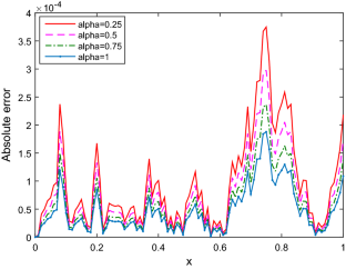
This paper is concerned with numerical solution of time fractional stochastic advection-diffusion type equation where the first order derivative is substituted by a Caputo fractional derivative of order \(\alpha \) ( \(0 <\alpha \le 1\) ). This type of equations due to randomness can rarely be solved, exactly. In this paper, a new approach based on finite difference method and spline approximation is employed to solve time fractional stochastic advection-diffusion type equation, numerically. After implementation of proposed method, the under consideration equation is transformed to a system of second order differential equations with appropriate boundary conditions. Then, using a suitable numerical method such as the backward differentiation formula, the resulting system can be solved. In addition, the error analysis is shown in some mild conditions by ignoring the error terms \(O(\Delta t^2)\) in the system. In order to show the pertinent features of the suggested algorithm such as accuracy, efficiency and reliability, some test problems are included. Comparison achieved results via proposed scheme in the case of classical stochastic advection-diffusion equation ( \(\alpha =1\) ) with obtained results via wavelets Galerkin method and obtained results for other values of \(\alpha \) with the values of exact solution confirm the validity, efficiency and applicability of the proposed method.

This is a preview of subscription content, log in via an institution to check access.

Access this article

Price includes VAT (Russian Federation)

Instant access to the full article PDF.

Rent this article via DeepDyve

Institutional subscriptions

Similar content being viewed by others

Analyses of the Contour Integral Method for Time Fractional Normal-Subdiffusion Transport Equation

Fugui Ma, Lijing Zhao, … Yejuan Wang

Numerical analysis for optimal quadratic spline collocation method in two space dimensions with application to nonlinear time-fractional diffusion equation

Xiao Ye, Xiangcheng Zheng, … Yue Liu

Numerical approach for time-fractional Burgers’ equation via a combination of Adams–Moulton and linearized technique

Yonghyeon Jeon & Sunyoung Bu

Abbasbandy S, Kazem S, Alhuthali MS, Alsulami HH (2015) Application of the operational matrix of fractional-order Legendre functions for solving the time-fractional convection-diffusion equation. Appl Math Comput 266:31–40

MathSciNet   MATH   Google Scholar  

Ahmadi N, Vahidi AR, Allahviranloo T (2017) An efficient approach based on radial basis functions for solving stochastic fractional differential equations. Math Sci 11:113–118

Article   MathSciNet   Google Scholar  

Babaei A, Jafari H, Ahmadi M (2019) A fractional order HIV/AIDS model based on the effect of screening of unaware infectives. Math Methods Appl Sci 42(7):2334–2343

Badr M, Yazdani A, Jafari H (2018) Stability of a finite volume element method for the time-fractional advection-diffusion equation. Numer Methods Partial Differ Equ 34(5):1459–1471

Baeumer B, Kovács M, Meerschaert MM (2008) Numerical solutions for fractional reaction-diffusion equations. Comput Math Appl 55(10):2212–2226

Baleanu D, Diethelm K, Scalas E, Trujillo J (2012) Fractional calculus models and numerical methods. Series on Complexity, Nonlinearity and Chaos. World Scientific, Singapore

Book   Google Scholar  

Dehghan M, Shirzadi M (2015) meshless simulation of stochastic advection-diffusion equations based on radial basis functions. Eng Anal Bound Elem 53:18–26

Firoozjaee MA, Jafari H, Lia A, Baleanu D (2018) Numerical approach of Fokker–Planck equation with Caputo–Fabrizio fractional derivative using Ritz approximation. J Comput Appl Math 339:367–373

Heydari MH, Avazzadeh Z (2018) An operational matrix method for solving variable-order fractional biharmonic equation. Comput Appl Math 37(4):4397–4411

Heydari MH, Hooshmandasl MR, Maalek Ghaini FM, Cattani C (2014) A computational method for solving stochastic Itô–Volterra integral equations based on stochastic operational matrix for generalized hat basis functions. J Comput Phys 270:402–415

Heydari MH, Hooshmandasl MR, Barid Loghmani G, Cattani C (2016) Wavelets Galerkin method for solving stochastic heat equation. Int J Comput Math 93.9:1579–1596

Kamrani M, Jamshidi N (2017) Implicit Euler approximation of stochastic evolution equations with fractional Brownian motion. Commun Nonlinear Sci Numer Simulat 44:1–10

Khodabin M, Maleknejad K, Fallahpour M (2015) Approximation solution of two-dimensional linear stochastic Fredholm integral equation by applying the Haar wavelet. Int J Math Model Comput 5(4):361–372

Google Scholar  

Li C, Zeng F (2013) The finite difference methods for fractional ordinary differential equations. Numer Funct Anal Opt 34.2:149–179

Li C, Chen A, Ye J (2011) Numerical approaches to fractional calculus and fractional ordinary differential equation. J Comput Phys 230(9):3352–3368

Liu F, Zhuang P, Anh V, Turner I, Burrage K (2007) Stability and convergence of the difference methods for the space-time fractional advection-diffusion equation. Appl Math Comput 191(1):12–20

Mirzaee F, Samadyar N (2017) Application of operational matrices for solving system of linear Stratonovich Volterra integral equation. J Comput Appl Math 320:164–175

Mirzaee F, Samadyar N (2017) Application of orthonormal Bernstein polynomials to construct a efficient scheme for solving fractional stochastic integro-differential equation. Optik Int J Light Electron Opt 132:262–273

Article   Google Scholar  

Mirzaee F, Samadyar N (2018) Using radial basis functions to solve two dimensional linear stochastic integral equations on non-rectangular domains. Eng Anal Bound Elem 92:180–195

Mirzaee F, Samadyar N (2019) On the numerical solution of fractional stochastic integro-differential equations via meshless discrete collocation method based on radial basis functions. Eng Anal Bound Anal 100:246–255

Mirzaee F, Samadyar N (2018) On the numerical method for solving a system of nonlinear fractional ordinary differential equations arising in HIV infection of CD4 \(^+\) T cells. Iran J Sci Technol Trans Sci 1–12

Ollivier-Gooch C, Van Altena M (2002) A high-order-accurate unstructured mesh finite-volume scheme for the advection-diffusion equation. J Comput Phys 181(2):729–752

Prieto FU, Muñoz JJB, Corvinos LG (2011) Application of the generalized finite difference method to solve the advection-diffusion equation. J Comput Appl Math 235(7):1849–1855

Roop JP (2008) Numerical approximation of a one-dimensional space fractional advection-dispersion equation with boundary layer. Comput Math Appl 56(7):1808–1819

Salehi Y, Darvishi MT, Schiesser WE (2018) Numerical solution of space fractional diffusion equation by the method of lines and splines. Appl Math Comput 336:465–480

Servan-Camas B, Tsai FTC (2008) Lattice Boltzmann method with two relaxation times for advection-diffusion equation: third order analysis and stability analysis. Adv Water Resour 31(8):1113–1126

Singh A, Das S, Ong SH, Jafari H (2019) Numerical solution of nonlinear reaction-advection-diffusion equation. J Comput Nonlinear Dyn 14(4):041003

Sousa E (2009) Finite difference approximations for a fractional advection diffusion problem. J Comput Phys 228(11):4038–4054

Sousa E (2011) Numerical approximations for fractional diffusion equations via splines. Comput Math Appl 62(3):938–944

Sousa E, Li C (2015) A weighted finite difference method for the fractional diffusion equation based on the Riemann–Liouville derivative. Appl Numer Math 90:22–37

Su L, Wang W, Wang H (2011) A characteristic difference method for the transient fractional convection-diffusion equations. Appl Numer Math 61(8):946–960

Taheri Z, Javadi S, Babolian E (2017) Numerical solution of stochastic fractional integro-differential equation by the spectral collocation method. J Comput Appl Math 321:336–347

Yang Q, Liu F, Turner I (2010) Numerical methods for fractional partial differential equations with Riesz space fractional derivatives. Appl Math Model 34(1):200–218

Zheng Y, Li C, Zhao Z (2010) A note on the finite element method for the space-fractional advection diffusion equation. Comput Math Appl 59(5):1718–1726

Zhuang P, Liu F, Anh V, Turner I (2009) Numerical methods for the variable-order fractional advection-diffusion equation with a nonlinear source term. SIAM J Numer Anal 47(3):1760–1781

Zhuang P, Gu Y, Liu F, Turner I, Yarlagadda PKDV (2011) Time-dependent fractional advection-diffusion equations by an implicit MLS meshless method. Int J Numer Methods Eng 88(13):1346–1362

Download references

Acknowledgements

The authors would like to state our appreciation to the editor and referees for their costly comments and constructive suggestions which have improved the quality of the current paper.

Author information

Authors and affiliations.

Faculty of Mathematical Sciences and Statistics, Malayer University, P. O. Box 65719-95863, Malayer, Iran

Farshid Mirzaee, Khosro Sayevand, Shadi Rezaei & Nasrin Samadyar

You can also search for this author in PubMed   Google Scholar

Corresponding author

Correspondence to Farshid Mirzaee .

Rights and permissions

Reprints and permissions

About this article

Mirzaee, F., Sayevand, K., Rezaei, S. et al. Finite Difference and Spline Approximation for Solving Fractional Stochastic Advection-Diffusion Equation. Iran J Sci Technol Trans Sci 45 , 607–617 (2021). https://doi.org/10.1007/s40995-020-01036-6

Download citation

Received : 02 April 2020

Accepted : 11 November 2020

Published : 27 November 2020

Issue Date : April 2021

DOI : https://doi.org/10.1007/s40995-020-01036-6

Share this article

Anyone you share the following link with will be able to read this content:

Sorry, a shareable link is not currently available for this article.

Provided by the Springer Nature SharedIt content-sharing initiative

• Fractional stochastic advection-diffusion equation
• Stochastic partial differential equations
• Caputo fractional derivative
• Finite difference method
• Spline approximation
• Brownian motion process

Mathematics Subject Classification

Advertisement

• Find a journal
• Publish with us
• Track your research

Academia.edu no longer supports Internet Explorer.

To browse Academia.edu and the wider internet faster and more securely, please take a few seconds to  upgrade your browser .

•  We're Hiring!
•  Help Center

Finite-Difference Methods

• Most Cited Papers
• Most Downloaded Papers
• Newest Papers
• Save to Library
• Last »
• Finite Volume Methods Follow Following
• Finite Difference Method Follow Following
• Multiscale computational models Follow Following
• Conservation Laws Follow Following
• Comsol Multiphysics Simulation Follow Following
• Liquid Crystals Follow Following
• Statistical Signal Processing Follow Following
• Residual Stress (Engineering) Follow Following
• Cell Phones Follow Following
• Partial Differential Equations Follow Following

Enter the email address you signed up with and we'll email you a reset link.

• Academia.edu Publishing
•   We're Hiring!
•   Help Center
• Find new research papers in:
• Health Sciences
• Earth Sciences
• Cognitive Science
• Mathematics
• Computer Science
• Academia ©2024