Want to create or adapt books like this? Learn more about how Pressbooks supports open publishing practices.
Chapter 13: Inferential Statistics

Understanding Null Hypothesis Testing
Learning Objectives
- Explain the purpose of null hypothesis testing, including the role of sampling error.
- Describe the basic logic of null hypothesis testing.
- Describe the role of relationship strength and sample size in determining statistical significance and make reasonable judgments about statistical significance based on these two factors.
The Purpose of Null Hypothesis Testing
As we have seen, psychological research typically involves measuring one or more variables for a sample and computing descriptive statistics for that sample. In general, however, the researcher’s goal is not to draw conclusions about that sample but to draw conclusions about the population that the sample was selected from. Thus researchers must use sample statistics to draw conclusions about the corresponding values in the population. These corresponding values in the population are called parameters . Imagine, for example, that a researcher measures the number of depressive symptoms exhibited by each of 50 clinically depressed adults and computes the mean number of symptoms. The researcher probably wants to use this sample statistic (the mean number of symptoms for the sample) to draw conclusions about the corresponding population parameter (the mean number of symptoms for clinically depressed adults).
Unfortunately, sample statistics are not perfect estimates of their corresponding population parameters. This is because there is a certain amount of random variability in any statistic from sample to sample. The mean number of depressive symptoms might be 8.73 in one sample of clinically depressed adults, 6.45 in a second sample, and 9.44 in a third—even though these samples are selected randomly from the same population. Similarly, the correlation (Pearson’s r ) between two variables might be +.24 in one sample, −.04 in a second sample, and +.15 in a third—again, even though these samples are selected randomly from the same population. This random variability in a statistic from sample to sample is called sampling error . (Note that the term error here refers to random variability and does not imply that anyone has made a mistake. No one “commits a sampling error.”)
One implication of this is that when there is a statistical relationship in a sample, it is not always clear that there is a statistical relationship in the population. A small difference between two group means in a sample might indicate that there is a small difference between the two group means in the population. But it could also be that there is no difference between the means in the population and that the difference in the sample is just a matter of sampling error. Similarly, a Pearson’s r value of −.29 in a sample might mean that there is a negative relationship in the population. But it could also be that there is no relationship in the population and that the relationship in the sample is just a matter of sampling error.
In fact, any statistical relationship in a sample can be interpreted in two ways:
- There is a relationship in the population, and the relationship in the sample reflects this.
- There is no relationship in the population, and the relationship in the sample reflects only sampling error.
The purpose of null hypothesis testing is simply to help researchers decide between these two interpretations.
The Logic of Null Hypothesis Testing
Null hypothesis testing is a formal approach to deciding between two interpretations of a statistical relationship in a sample. One interpretation is called the null hypothesis (often symbolized H 0 and read as “H-naught”). This is the idea that there is no relationship in the population and that the relationship in the sample reflects only sampling error. Informally, the null hypothesis is that the sample relationship “occurred by chance.” The other interpretation is called the alternative hypothesis (often symbolized as H 1 ). This is the idea that there is a relationship in the population and that the relationship in the sample reflects this relationship in the population.
Again, every statistical relationship in a sample can be interpreted in either of these two ways: It might have occurred by chance, or it might reflect a relationship in the population. So researchers need a way to decide between them. Although there are many specific null hypothesis testing techniques, they are all based on the same general logic. The steps are as follows:
- Assume for the moment that the null hypothesis is true. There is no relationship between the variables in the population.
- Determine how likely the sample relationship would be if the null hypothesis were true.
- If the sample relationship would be extremely unlikely, then reject the null hypothesis in favour of the alternative hypothesis. If it would not be extremely unlikely, then retain the null hypothesis .
Following this logic, we can begin to understand why Mehl and his colleagues concluded that there is no difference in talkativeness between women and men in the population. In essence, they asked the following question: “If there were no difference in the population, how likely is it that we would find a small difference of d = 0.06 in our sample?” Their answer to this question was that this sample relationship would be fairly likely if the null hypothesis were true. Therefore, they retained the null hypothesis—concluding that there is no evidence of a sex difference in the population. We can also see why Kanner and his colleagues concluded that there is a correlation between hassles and symptoms in the population. They asked, “If the null hypothesis were true, how likely is it that we would find a strong correlation of +.60 in our sample?” Their answer to this question was that this sample relationship would be fairly unlikely if the null hypothesis were true. Therefore, they rejected the null hypothesis in favour of the alternative hypothesis—concluding that there is a positive correlation between these variables in the population.
A crucial step in null hypothesis testing is finding the likelihood of the sample result if the null hypothesis were true. This probability is called the p value . A low p value means that the sample result would be unlikely if the null hypothesis were true and leads to the rejection of the null hypothesis. A high p value means that the sample result would be likely if the null hypothesis were true and leads to the retention of the null hypothesis. But how low must the p value be before the sample result is considered unlikely enough to reject the null hypothesis? In null hypothesis testing, this criterion is called α (alpha) and is almost always set to .05. If there is less than a 5% chance of a result as extreme as the sample result if the null hypothesis were true, then the null hypothesis is rejected. When this happens, the result is said to be statistically significant . If there is greater than a 5% chance of a result as extreme as the sample result when the null hypothesis is true, then the null hypothesis is retained. This does not necessarily mean that the researcher accepts the null hypothesis as true—only that there is not currently enough evidence to conclude that it is true. Researchers often use the expression “fail to reject the null hypothesis” rather than “retain the null hypothesis,” but they never use the expression “accept the null hypothesis.”
The Misunderstood p Value
The p value is one of the most misunderstood quantities in psychological research (Cohen, 1994) [1] . Even professional researchers misinterpret it, and it is not unusual for such misinterpretations to appear in statistics textbooks!
The most common misinterpretation is that the p value is the probability that the null hypothesis is true—that the sample result occurred by chance. For example, a misguided researcher might say that because the p value is .02, there is only a 2% chance that the result is due to chance and a 98% chance that it reflects a real relationship in the population. But this is incorrect . The p value is really the probability of a result at least as extreme as the sample result if the null hypothesis were true. So a p value of .02 means that if the null hypothesis were true, a sample result this extreme would occur only 2% of the time.
You can avoid this misunderstanding by remembering that the p value is not the probability that any particular hypothesis is true or false. Instead, it is the probability of obtaining the sample result if the null hypothesis were true.
Role of Sample Size and Relationship Strength
Recall that null hypothesis testing involves answering the question, “If the null hypothesis were true, what is the probability of a sample result as extreme as this one?” In other words, “What is the p value?” It can be helpful to see that the answer to this question depends on just two considerations: the strength of the relationship and the size of the sample. Specifically, the stronger the sample relationship and the larger the sample, the less likely the result would be if the null hypothesis were true. That is, the lower the p value. This should make sense. Imagine a study in which a sample of 500 women is compared with a sample of 500 men in terms of some psychological characteristic, and Cohen’s d is a strong 0.50. If there were really no sex difference in the population, then a result this strong based on such a large sample should seem highly unlikely. Now imagine a similar study in which a sample of three women is compared with a sample of three men, and Cohen’s d is a weak 0.10. If there were no sex difference in the population, then a relationship this weak based on such a small sample should seem likely. And this is precisely why the null hypothesis would be rejected in the first example and retained in the second.
Of course, sometimes the result can be weak and the sample large, or the result can be strong and the sample small. In these cases, the two considerations trade off against each other so that a weak result can be statistically significant if the sample is large enough and a strong relationship can be statistically significant even if the sample is small. Table 13.1 shows roughly how relationship strength and sample size combine to determine whether a sample result is statistically significant. The columns of the table represent the three levels of relationship strength: weak, medium, and strong. The rows represent four sample sizes that can be considered small, medium, large, and extra large in the context of psychological research. Thus each cell in the table represents a combination of relationship strength and sample size. If a cell contains the word Yes , then this combination would be statistically significant for both Cohen’s d and Pearson’s r . If it contains the word No , then it would not be statistically significant for either. There is one cell where the decision for d and r would be different and another where it might be different depending on some additional considerations, which are discussed in Section 13.2 “Some Basic Null Hypothesis Tests”
Although Table 13.1 provides only a rough guideline, it shows very clearly that weak relationships based on medium or small samples are never statistically significant and that strong relationships based on medium or larger samples are always statistically significant. If you keep this lesson in mind, you will often know whether a result is statistically significant based on the descriptive statistics alone. It is extremely useful to be able to develop this kind of intuitive judgment. One reason is that it allows you to develop expectations about how your formal null hypothesis tests are going to come out, which in turn allows you to detect problems in your analyses. For example, if your sample relationship is strong and your sample is medium, then you would expect to reject the null hypothesis. If for some reason your formal null hypothesis test indicates otherwise, then you need to double-check your computations and interpretations. A second reason is that the ability to make this kind of intuitive judgment is an indication that you understand the basic logic of this approach in addition to being able to do the computations.
Statistical Significance Versus Practical Significance
Table 13.1 illustrates another extremely important point. A statistically significant result is not necessarily a strong one. Even a very weak result can be statistically significant if it is based on a large enough sample. This is closely related to Janet Shibley Hyde’s argument about sex differences (Hyde, 2007) [2] . The differences between women and men in mathematical problem solving and leadership ability are statistically significant. But the word significant can cause people to interpret these differences as strong and important—perhaps even important enough to influence the college courses they take or even who they vote for. As we have seen, however, these statistically significant differences are actually quite weak—perhaps even “trivial.”
This is why it is important to distinguish between the statistical significance of a result and the practical significance of that result. Practical significance refers to the importance or usefulness of the result in some real-world context. Many sex differences are statistically significant—and may even be interesting for purely scientific reasons—but they are not practically significant. In clinical practice, this same concept is often referred to as “clinical significance.” For example, a study on a new treatment for social phobia might show that it produces a statistically significant positive effect. Yet this effect still might not be strong enough to justify the time, effort, and other costs of putting it into practice—especially if easier and cheaper treatments that work almost as well already exist. Although statistically significant, this result would be said to lack practical or clinical significance.
Key Takeaways
- Null hypothesis testing is a formal approach to deciding whether a statistical relationship in a sample reflects a real relationship in the population or is just due to chance.
- The logic of null hypothesis testing involves assuming that the null hypothesis is true, finding how likely the sample result would be if this assumption were correct, and then making a decision. If the sample result would be unlikely if the null hypothesis were true, then it is rejected in favour of the alternative hypothesis. If it would not be unlikely, then the null hypothesis is retained.
- The probability of obtaining the sample result if the null hypothesis were true (the p value) is based on two considerations: relationship strength and sample size. Reasonable judgments about whether a sample relationship is statistically significant can often be made by quickly considering these two factors.
- Statistical significance is not the same as relationship strength or importance. Even weak relationships can be statistically significant if the sample size is large enough. It is important to consider relationship strength and the practical significance of a result in addition to its statistical significance.
- Discussion: Imagine a study showing that people who eat more broccoli tend to be happier. Explain for someone who knows nothing about statistics why the researchers would conduct a null hypothesis test.
- The correlation between two variables is r = −.78 based on a sample size of 137.
- The mean score on a psychological characteristic for women is 25 ( SD = 5) and the mean score for men is 24 ( SD = 5). There were 12 women and 10 men in this study.
- In a memory experiment, the mean number of items recalled by the 40 participants in Condition A was 0.50 standard deviations greater than the mean number recalled by the 40 participants in Condition B.
- In another memory experiment, the mean scores for participants in Condition A and Condition B came out exactly the same!
- A student finds a correlation of r = .04 between the number of units the students in his research methods class are taking and the students’ level of stress.
Long Descriptions
“Null Hypothesis” long description: A comic depicting a man and a woman talking in the foreground. In the background is a child working at a desk. The man says to the woman, “I can’t believe schools are still teaching kids about the null hypothesis. I remember reading a big study that conclusively disproved it years ago.” [Return to “Null Hypothesis”]
“Conditional Risk” long description: A comic depicting two hikers beside a tree during a thunderstorm. A bolt of lightning goes “crack” in the dark sky as thunder booms. One of the hikers says, “Whoa! We should get inside!” The other hiker says, “It’s okay! Lightning only kills about 45 Americans a year, so the chances of dying are only one in 7,000,000. Let’s go on!” The comic’s caption says, “The annual death rate among people who know that statistic is one in six.” [Return to “Conditional Risk”]
Media Attributions
- Null Hypothesis by XKCD CC BY-NC (Attribution NonCommercial)
- Conditional Risk by XKCD CC BY-NC (Attribution NonCommercial)
- Cohen, J. (1994). The world is round: p < .05. American Psychologist, 49 , 997–1003. ↵
- Hyde, J. S. (2007). New directions in the study of gender similarities and differences. Current Directions in Psychological Science, 16 , 259–263. ↵
Values in a population that correspond to variables measured in a study.
The random variability in a statistic from sample to sample.
A formal approach to deciding between two interpretations of a statistical relationship in a sample.
The idea that there is no relationship in the population and that the relationship in the sample reflects only sampling error.
The idea that there is a relationship in the population and that the relationship in the sample reflects this relationship in the population.
When the relationship found in the sample would be extremely unlikely, the idea that the relationship occurred “by chance” is rejected.
When the relationship found in the sample is likely to have occurred by chance, the null hypothesis is not rejected.
The probability that, if the null hypothesis were true, the result found in the sample would occur.
How low the p value must be before the sample result is considered unlikely in null hypothesis testing.
When there is less than a 5% chance of a result as extreme as the sample result occurring and the null hypothesis is rejected.
Research Methods in Psychology - 2nd Canadian Edition Copyright © 2015 by Paul C. Price, Rajiv Jhangiani, & I-Chant A. Chiang is licensed under a Creative Commons Attribution-NonCommercial-ShareAlike 4.0 International License , except where otherwise noted.
Share This Book

Want to create or adapt books like this? Learn more about how Pressbooks supports open publishing practices.
Inferential Statistics
Learning Objectives
- Explain the purpose of null hypothesis testing, including the role of sampling error.
- Describe the basic logic of null hypothesis testing.
- Describe the role of relationship strength and sample size in determining statistical significance and make reasonable judgments about statistical significance based on these two factors.
The Purpose of Null Hypothesis Testing
As we have seen, psychological research typically involves measuring one or more variables in a sample and computing descriptive summary data (e.g., means, correlation coefficients) for those variables. These descriptive data for the sample are called statistics . In general, however, the researcher’s goal is not to draw conclusions about that sample but to draw conclusions about the population that the sample was selected from. Thus researchers must use sample statistics to draw conclusions about the corresponding values in the population. These corresponding values in the population are called parameters . Imagine, for example, that a researcher measures the number of depressive symptoms exhibited by each of 50 adults with clinical depression and computes the mean number of symptoms. The researcher probably wants to use this sample statistic (the mean number of symptoms for the sample) to draw conclusions about the corresponding population parameter (the mean number of symptoms for adults with clinical depression).
Unfortunately, sample statistics are not perfect estimates of their corresponding population parameters. This is because there is a certain amount of random variability in any statistic from sample to sample. The mean number of depressive symptoms might be 8.73 in one sample of adults with clinical depression, 6.45 in a second sample, and 9.44 in a third—even though these samples are selected randomly from the same population. Similarly, the correlation (Pearson’s r ) between two variables might be +.24 in one sample, −.04 in a second sample, and +.15 in a third—again, even though these samples are selected randomly from the same population. This random variability in a statistic from sample to sample is called sampling error . (Note that the term error here refers to random variability and does not imply that anyone has made a mistake. No one “commits a sampling error.”)
One implication of this is that when there is a statistical relationship in a sample, it is not always clear that there is a statistical relationship in the population. A small difference between two group means in a sample might indicate that there is a small difference between the two group means in the population. But it could also be that there is no difference between the means in the population and that the difference in the sample is just a matter of sampling error. Similarly, a Pearson’s r value of −.29 in a sample might mean that there is a negative relationship in the population. But it could also be that there is no relationship in the population and that the relationship in the sample is just a matter of sampling error.
In fact, any statistical relationship in a sample can be interpreted in two ways:
- There is a relationship in the population, and the relationship in the sample reflects this.
- There is no relationship in the population, and the relationship in the sample reflects only sampling error.
The purpose of null hypothesis testing is simply to help researchers decide between these two interpretations.
The Logic of Null Hypothesis Testing
Null hypothesis testing (often called null hypothesis significance testing or NHST) is a formal approach to deciding between two interpretations of a statistical relationship in a sample. One interpretation is called the null hypothesis (often symbolized H 0 and read as “H-zero”). This is the idea that there is no relationship in the population and that the relationship in the sample reflects only sampling error. Informally, the null hypothesis is that the sample relationship “occurred by chance.” The other interpretation is called the alternative hypothesis (often symbolized as H 1 ). This is the idea that there is a relationship in the population and that the relationship in the sample reflects this relationship in the population.
Again, every statistical relationship in a sample can be interpreted in either of these two ways: It might have occurred by chance, or it might reflect a relationship in the population. So researchers need a way to decide between them. Although there are many specific null hypothesis testing techniques, they are all based on the same general logic. The steps are as follows:
- Assume for the moment that the null hypothesis is true. There is no relationship between the variables in the population.
- Determine how likely the sample relationship would be if the null hypothesis were true.
- If the sample relationship would be extremely unlikely, then reject the null hypothesis in favor of the alternative hypothesis. If it would not be extremely unlikely, then retain the null hypothesis .
Following this logic, we can begin to understand why Mehl and his colleagues concluded that there is no difference in talkativeness between women and men in the population. In essence, they asked the following question: “If there were no difference in the population, how likely is it that we would find a small difference of d = 0.06 in our sample?” Their answer to this question was that this sample relationship would be fairly likely if the null hypothesis were true. Therefore, they retained the null hypothesis—concluding that there is no evidence of a sex difference in the population. We can also see why Kanner and his colleagues concluded that there is a correlation between hassles and symptoms in the population. They asked, “If the null hypothesis were true, how likely is it that we would find a strong correlation of +.60 in our sample?” Their answer to this question was that this sample relationship would be fairly unlikely if the null hypothesis were true. Therefore, they rejected the null hypothesis in favor of the alternative hypothesis—concluding that there is a positive correlation between these variables in the population.
A crucial step in null hypothesis testing is finding the probability of the sample result or a more extreme result if the null hypothesis were true (Lakens, 2017). [1] This probability is called the p value . A low p value means that the sample or more extreme result would be unlikely if the null hypothesis were true and leads to the rejection of the null hypothesis. A p value that is not low means that the sample or more extreme result would be likely if the null hypothesis were true and leads to the retention of the null hypothesis. But how low must the p value criterion be before the sample result is considered unlikely enough to reject the null hypothesis? In null hypothesis testing, this criterion is called α (alpha) and is almost always set to .05. If there is a 5% chance or less of a result at least as extreme as the sample result if the null hypothesis were true, then the null hypothesis is rejected. When this happens, the result is said to be statistically significant . If there is greater than a 5% chance of a result as extreme as the sample result when the null hypothesis is true, then the null hypothesis is retained. This does not necessarily mean that the researcher accepts the null hypothesis as true—only that there is not currently enough evidence to reject it. Researchers often use the expression “fail to reject the null hypothesis” rather than “retain the null hypothesis,” but they never use the expression “accept the null hypothesis.”
The Misunderstood p Value
The p value is one of the most misunderstood quantities in psychological research (Cohen, 1994) [2] . Even professional researchers misinterpret it, and it is not unusual for such misinterpretations to appear in statistics textbooks!
The most common misinterpretation is that the p value is the probability that the null hypothesis is true—that the sample result occurred by chance. For example, a misguided researcher might say that because the p value is .02, there is only a 2% chance that the result is due to chance and a 98% chance that it reflects a real relationship in the population. But this is incorrect . The p value is really the probability of a result at least as extreme as the sample result if the null hypothesis were true. So a p value of .02 means that if the null hypothesis were true, a sample result this extreme would occur only 2% of the time.
You can avoid this misunderstanding by remembering that the p value is not the probability that any particular hypothesis is true or false. Instead, it is the probability of obtaining the sample result if the null hypothesis were true.

Role of Sample Size and Relationship Strength
Recall that null hypothesis testing involves answering the question, “If the null hypothesis were true, what is the probability of a sample result as extreme as this one?” In other words, “What is the p value?” It can be helpful to see that the answer to this question depends on just two considerations: the strength of the relationship and the size of the sample. Specifically, the stronger the sample relationship and the larger the sample, the less likely the result would be if the null hypothesis were true. That is, the lower the p value. This should make sense. Imagine a study in which a sample of 500 women is compared with a sample of 500 men in terms of some psychological characteristic, and Cohen’s d is a strong 0.50. If there were really no sex difference in the population, then a result this strong based on such a large sample should seem highly unlikely. Now imagine a similar study in which a sample of three women is compared with a sample of three men, and Cohen’s d is a weak 0.10. If there were no sex difference in the population, then a relationship this weak based on such a small sample should seem likely. And this is precisely why the null hypothesis would be rejected in the first example and retained in the second.
Of course, sometimes the result can be weak and the sample large, or the result can be strong and the sample small. In these cases, the two considerations trade off against each other so that a weak result can be statistically significant if the sample is large enough and a strong relationship can be statistically significant even if the sample is small. Table 13.1 shows roughly how relationship strength and sample size combine to determine whether a sample result is statistically significant. The columns of the table represent the three levels of relationship strength: weak, medium, and strong. The rows represent four sample sizes that can be considered small, medium, large, and extra large in the context of psychological research. Thus each cell in the table represents a combination of relationship strength and sample size. If a cell contains the word Yes , then this combination would be statistically significant for both Cohen’s d and Pearson’s r . If it contains the word No , then it would not be statistically significant for either. There is one cell where the decision for d and r would be different and another where it might be different depending on some additional considerations, which are discussed in Section 13.2 “Some Basic Null Hypothesis Tests”
Although Table 13.1 provides only a rough guideline, it shows very clearly that weak relationships based on medium or small samples are never statistically significant and that strong relationships based on medium or larger samples are always statistically significant. If you keep this lesson in mind, you will often know whether a result is statistically significant based on the descriptive statistics alone. It is extremely useful to be able to develop this kind of intuitive judgment. One reason is that it allows you to develop expectations about how your formal null hypothesis tests are going to come out, which in turn allows you to detect problems in your analyses. For example, if your sample relationship is strong and your sample is medium, then you would expect to reject the null hypothesis. If for some reason your formal null hypothesis test indicates otherwise, then you need to double-check your computations and interpretations. A second reason is that the ability to make this kind of intuitive judgment is an indication that you understand the basic logic of this approach in addition to being able to do the computations.
Statistical Significance Versus Practical Significance
Table 13.1 illustrates another extremely important point. A statistically significant result is not necessarily a strong one. Even a very weak result can be statistically significant if it is based on a large enough sample. This is closely related to Janet Shibley Hyde’s argument about sex differences (Hyde, 2007) [3] . The differences between women and men in mathematical problem solving and leadership ability are statistically significant. But the word significant can cause people to interpret these differences as strong and important—perhaps even important enough to influence the college courses they take or even who they vote for. As we have seen, however, these statistically significant differences are actually quite weak—perhaps even “trivial.”
This is why it is important to distinguish between the statistical significance of a result and the practical significance of that result. Practical significance refers to the importance or usefulness of the result in some real-world context. Many sex differences are statistically significant—and may even be interesting for purely scientific reasons—but they are not practically significant. In clinical practice, this same concept is often referred to as “clinical significance.” For example, a study on a new treatment for social phobia might show that it produces a statistically significant positive effect. Yet this effect still might not be strong enough to justify the time, effort, and other costs of putting it into practice—especially if easier and cheaper treatments that work almost as well already exist. Although statistically significant, this result would be said to lack practical or clinical significance.

Image Description
“Null Hypothesis” long description: A comic depicting a man and a woman talking in the foreground. In the background is a child working at a desk. The man says to the woman, “I can’t believe schools are still teaching kids about the null hypothesis. I remember reading a big study that conclusively disproved it years ago.” [Return to “Null Hypothesis”]
“Conditional Risk” long description: A comic depicting two hikers beside a tree during a thunderstorm. A bolt of lightning goes “crack” in the dark sky as thunder booms. One of the hikers says, “Whoa! We should get inside!” The other hiker says, “It’s okay! Lightning only kills about 45 Americans a year, so the chances of dying are only one in 7,000,000. Let’s go on!” The comic’s caption says, “The annual death rate among people who know that statistic is one in six.” [Return to “Conditional Risk”]
Media Attributions
- Null Hypothesis by XKCD CC BY-NC (Attribution NonCommercial)
- Conditional Risk by XKCD CC BY-NC (Attribution NonCommercial)
- Lakens, D. (2017, December 25). About p -values: Understanding common misconceptions. [Blog post] Retrieved from https://correlaid.org/en/blog/understand-p-values/ ↵
- Cohen, J. (1994). The world is round: p < .05. American Psychologist, 49 , 997–1003. ↵
- Hyde, J. S. (2007). New directions in the study of gender similarities and differences. Current Directions in Psychological Science, 16 , 259–263. ↵
Descriptive data that involves measuring one or more variables in a sample and computing descriptive summary data (e.g., means, correlation coefficients) for those variables.
Corresponding values in the population.
The random variability in a statistic from sample to sample.
A formal approach to deciding between two interpretations of a statistical relationship in a sample.
The idea that there is no relationship in the population and that the relationship in the sample reflects only sampling error (often symbolized H0 and read as “H-zero”).
An alternative to the null hypothesis (often symbolized as H1), this hypothesis proposes that there is a relationship in the population and that the relationship in the sample reflects this relationship in the population.
A decision made by researchers using null hypothesis testing which occurs when the sample relationship would be extremely unlikely.
A decision made by researchers in null hypothesis testing which occurs when the sample relationship would not be extremely unlikely.
The probability of obtaining the sample result or a more extreme result if the null hypothesis were true.
The criterion that shows how low a p-value should be before the sample result is considered unlikely enough to reject the null hypothesis (Usually set to .05).
An effect that is unlikely due to random chance and therefore likely represents a real effect in the population.
Refers to the importance or usefulness of the result in some real-world context.
Research Methods in Psychology Copyright © 2019 by Rajiv S. Jhangiani, I-Chant A. Chiang, Carrie Cuttler, & Dana C. Leighton is licensed under a Creative Commons Attribution-NonCommercial-ShareAlike 4.0 International License , except where otherwise noted.
Share This Book

- school Campus Bookshelves
- menu_book Bookshelves
- perm_media Learning Objects
- login Login
- how_to_reg Request Instructor Account
- hub Instructor Commons
- Download Page (PDF)
- Download Full Book (PDF)
- Periodic Table
- Physics Constants
- Scientific Calculator
- Reference & Cite
- Tools expand_more
- Readability
selected template will load here
This action is not available.
9.1: Null and Alternative Hypotheses
- Last updated
- Save as PDF
- Page ID 23459

The actual test begins by considering two hypotheses . They are called the null hypothesis and the alternative hypothesis . These hypotheses contain opposing viewpoints.
\(H_0\): The null hypothesis: It is a statement of no difference between the variables—they are not related. This can often be considered the status quo and as a result if you cannot accept the null it requires some action.
\(H_a\): The alternative hypothesis: It is a claim about the population that is contradictory to \(H_0\) and what we conclude when we reject \(H_0\). This is usually what the researcher is trying to prove.
Since the null and alternative hypotheses are contradictory, you must examine evidence to decide if you have enough evidence to reject the null hypothesis or not. The evidence is in the form of sample data.
After you have determined which hypothesis the sample supports, you make a decision. There are two options for a decision. They are "reject \(H_0\)" if the sample information favors the alternative hypothesis or "do not reject \(H_0\)" or "decline to reject \(H_0\)" if the sample information is insufficient to reject the null hypothesis.
\(H_{0}\) always has a symbol with an equal in it. \(H_{a}\) never has a symbol with an equal in it. The choice of symbol depends on the wording of the hypothesis test. However, be aware that many researchers (including one of the co-authors in research work) use = in the null hypothesis, even with > or < as the symbol in the alternative hypothesis. This practice is acceptable because we only make the decision to reject or not reject the null hypothesis.
Example \(\PageIndex{1}\)
- \(H_{0}\): No more than 30% of the registered voters in Santa Clara County voted in the primary election. \(p \leq 30\)
- \(H_{a}\): More than 30% of the registered voters in Santa Clara County voted in the primary election. \(p > 30\)
Exercise \(\PageIndex{1}\)
A medical trial is conducted to test whether or not a new medicine reduces cholesterol by 25%. State the null and alternative hypotheses.
- \(H_{0}\): The drug reduces cholesterol by 25%. \(p = 0.25\)
- \(H_{a}\): The drug does not reduce cholesterol by 25%. \(p \neq 0.25\)
Example \(\PageIndex{2}\)
We want to test whether the mean GPA of students in American colleges is different from 2.0 (out of 4.0). The null and alternative hypotheses are:
- \(H_{0}: \mu = 2.0\)
- \(H_{a}: \mu \neq 2.0\)
Exercise \(\PageIndex{2}\)
We want to test whether the mean height of eighth graders is 66 inches. State the null and alternative hypotheses. Fill in the correct symbol \((=, \neq, \geq, <, \leq, >)\) for the null and alternative hypotheses.
- \(H_{0}: \mu \_ 66\)
- \(H_{a}: \mu \_ 66\)
- \(H_{0}: \mu = 66\)
- \(H_{a}: \mu \neq 66\)
Example \(\PageIndex{3}\)
We want to test if college students take less than five years to graduate from college, on the average. The null and alternative hypotheses are:
- \(H_{0}: \mu \geq 5\)
- \(H_{a}: \mu < 5\)
Exercise \(\PageIndex{3}\)
We want to test if it takes fewer than 45 minutes to teach a lesson plan. State the null and alternative hypotheses. Fill in the correct symbol ( =, ≠, ≥, <, ≤, >) for the null and alternative hypotheses.
- \(H_{0}: \mu \_ 45\)
- \(H_{a}: \mu \_ 45\)
- \(H_{0}: \mu \geq 45\)
- \(H_{a}: \mu < 45\)
Example \(\PageIndex{4}\)
In an issue of U. S. News and World Report , an article on school standards stated that about half of all students in France, Germany, and Israel take advanced placement exams and a third pass. The same article stated that 6.6% of U.S. students take advanced placement exams and 4.4% pass. Test if the percentage of U.S. students who take advanced placement exams is more than 6.6%. State the null and alternative hypotheses.
- \(H_{0}: p \leq 0.066\)
- \(H_{a}: p > 0.066\)
Exercise \(\PageIndex{4}\)
On a state driver’s test, about 40% pass the test on the first try. We want to test if more than 40% pass on the first try. Fill in the correct symbol (\(=, \neq, \geq, <, \leq, >\)) for the null and alternative hypotheses.
- \(H_{0}: p \_ 0.40\)
- \(H_{a}: p \_ 0.40\)
- \(H_{0}: p = 0.40\)
- \(H_{a}: p > 0.40\)
COLLABORATIVE EXERCISE
Bring to class a newspaper, some news magazines, and some Internet articles . In groups, find articles from which your group can write null and alternative hypotheses. Discuss your hypotheses with the rest of the class.
In a hypothesis test , sample data is evaluated in order to arrive at a decision about some type of claim. If certain conditions about the sample are satisfied, then the claim can be evaluated for a population. In a hypothesis test, we:
- Evaluate the null hypothesis , typically denoted with \(H_{0}\). The null is not rejected unless the hypothesis test shows otherwise. The null statement must always contain some form of equality \((=, \leq \text{or} \geq)\)
- Always write the alternative hypothesis , typically denoted with \(H_{a}\) or \(H_{1}\), using less than, greater than, or not equals symbols, i.e., \((\neq, >, \text{or} <)\).
- If we reject the null hypothesis, then we can assume there is enough evidence to support the alternative hypothesis.
- Never state that a claim is proven true or false. Keep in mind the underlying fact that hypothesis testing is based on probability laws; therefore, we can talk only in terms of non-absolute certainties.
Formula Review
\(H_{0}\) and \(H_{a}\) are contradictory.
- If \(\alpha \leq p\)-value, then do not reject \(H_{0}\).
- If\(\alpha > p\)-value, then reject \(H_{0}\).
\(\alpha\) is preconceived. Its value is set before the hypothesis test starts. The \(p\)-value is calculated from the data.References
Data from the National Institute of Mental Health. Available online at http://www.nimh.nih.gov/publicat/depression.cfm .
Want to create or adapt books like this? Learn more about how Pressbooks supports open publishing practices.
13.1 Understanding Null Hypothesis Testing
Learning objectives.
- Explain the purpose of null hypothesis testing, including the role of sampling error.
- Describe the basic logic of null hypothesis testing.
- Describe the role of relationship strength and sample size in determining statistical significance and make reasonable judgments about statistical significance based on these two factors.
The Purpose of Null Hypothesis Testing
As we have seen, psychological research typically involves measuring one or more variables for a sample and computing descriptive statistics for that sample. In general, however, the researcher’s goal is not to draw conclusions about that sample but to draw conclusions about the population that the sample was selected from. Thus researchers must use sample statistics to draw conclusions about the corresponding values in the population. These corresponding values in the population are called parameters . Imagine, for example, that a researcher measures the number of depressive symptoms exhibited by each of 50 clinically depressed adults and computes the mean number of symptoms. The researcher probably wants to use this sample statistic (the mean number of symptoms for the sample) to draw conclusions about the corresponding population parameter (the mean number of symptoms for clinically depressed adults).
Unfortunately, sample statistics are not perfect estimates of their corresponding population parameters. This is because there is a certain amount of random variability in any statistic from sample to sample. The mean number of depressive symptoms might be 8.73 in one sample of clinically depressed adults, 6.45 in a second sample, and 9.44 in a third—even though these samples are selected randomly from the same population. Similarly, the correlation (Pearson’s r ) between two variables might be +.24 in one sample, −.04 in a second sample, and +.15 in a third—again, even though these samples are selected randomly from the same population. This random variability in a statistic from sample to sample is called sampling error . (Note that the term error here refers to random variability and does not imply that anyone has made a mistake. No one “commits a sampling error.”)
One implication of this is that when there is a statistical relationship in a sample, it is not always clear that there is a statistical relationship in the population. A small difference between two group means in a sample might indicate that there is a small difference between the two group means in the population. But it could also be that there is no difference between the means in the population and that the difference in the sample is just a matter of sampling error. Similarly, a Pearson’s r value of −.29 in a sample might mean that there is a negative relationship in the population. But it could also be that there is no relationship in the population and that the relationship in the sample is just a matter of sampling error.
In fact, any statistical relationship in a sample can be interpreted in two ways:
- There is a relationship in the population, and the relationship in the sample reflects this.
- There is no relationship in the population, and the relationship in the sample reflects only sampling error.
The purpose of null hypothesis testing is simply to help researchers decide between these two interpretations.
The Logic of Null Hypothesis Testing
Null hypothesis testing is a formal approach to deciding between two interpretations of a statistical relationship in a sample. One interpretation is called the null hypothesis (often symbolized H 0 and read as “H-naught”). This is the idea that there is no relationship in the population and that the relationship in the sample reflects only sampling error. Informally, the null hypothesis is that the sample relationship “occurred by chance.” The other interpretation is called the alternative hypothesis (often symbolized as H 1 ). This is the idea that there is a relationship in the population and that the relationship in the sample reflects this relationship in the population.
Again, every statistical relationship in a sample can be interpreted in either of these two ways: It might have occurred by chance, or it might reflect a relationship in the population. So researchers need a way to decide between them. Although there are many specific null hypothesis testing techniques, they are all based on the same general logic. The steps are as follows:
- Assume for the moment that the null hypothesis is true. There is no relationship between the variables in the population.
- Determine how likely the sample relationship would be if the null hypothesis were true.
- If the sample relationship would be extremely unlikely, then reject the null hypothesis in favor of the alternative hypothesis. If it would not be extremely unlikely, then retain the null hypothesis .
Following this logic, we can begin to understand why Mehl and his colleagues concluded that there is no difference in talkativeness between women and men in the population. In essence, they asked the following question: “If there were no difference in the population, how likely is it that we would find a small difference of d = 0.06 in our sample?” Their answer to this question was that this sample relationship would be fairly likely if the null hypothesis were true. Therefore, they retained the null hypothesis—concluding that there is no evidence of a sex difference in the population. We can also see why Kanner and his colleagues concluded that there is a correlation between hassles and symptoms in the population. They asked, “If the null hypothesis were true, how likely is it that we would find a strong correlation of +.60 in our sample?” Their answer to this question was that this sample relationship would be fairly unlikely if the null hypothesis were true. Therefore, they rejected the null hypothesis in favor of the alternative hypothesis—concluding that there is a positive correlation between these variables in the population.
A crucial step in null hypothesis testing is finding the likelihood of the sample result if the null hypothesis were true. This probability is called the p value . A low p value means that the sample result would be unlikely if the null hypothesis were true and leads to the rejection of the null hypothesis. A high p value means that the sample result would be likely if the null hypothesis were true and leads to the retention of the null hypothesis. But how low must the p value be before the sample result is considered unlikely enough to reject the null hypothesis? In null hypothesis testing, this criterion is called α (alpha) and is almost always set to .05. If there is less than a 5% chance of a result as extreme as the sample result if the null hypothesis were true, then the null hypothesis is rejected. When this happens, the result is said to be statistically significant . If there is greater than a 5% chance of a result as extreme as the sample result when the null hypothesis is true, then the null hypothesis is retained. This does not necessarily mean that the researcher accepts the null hypothesis as true—only that there is not currently enough evidence to conclude that it is true. Researchers often use the expression “fail to reject the null hypothesis” rather than “retain the null hypothesis,” but they never use the expression “accept the null hypothesis.”
The Misunderstood p Value
The p value is one of the most misunderstood quantities in psychological research (Cohen, 1994). Even professional researchers misinterpret it, and it is not unusual for such misinterpretations to appear in statistics textbooks!
The most common misinterpretation is that the p value is the probability that the null hypothesis is true—that the sample result occurred by chance. For example, a misguided researcher might say that because the p value is .02, there is only a 2% chance that the result is due to chance and a 98% chance that it reflects a real relationship in the population. But this is incorrect . The p value is really the probability of a result at least as extreme as the sample result if the null hypothesis were true. So a p value of .02 means that if the null hypothesis were true, a sample result this extreme would occur only 2% of the time.
You can avoid this misunderstanding by remembering that the p value is not the probability that any particular hypothesis is true or false. Instead, it is the probability of obtaining the sample result if the null hypothesis were true.
Role of Sample Size and Relationship Strength
Recall that null hypothesis testing involves answering the question, “If the null hypothesis were true, what is the probability of a sample result as extreme as this one?” In other words, “What is the p value?” It can be helpful to see that the answer to this question depends on just two considerations: the strength of the relationship and the size of the sample. Specifically, the stronger the sample relationship and the larger the sample, the less likely the result would be if the null hypothesis were true. That is, the lower the p value. This should make sense. Imagine a study in which a sample of 500 women is compared with a sample of 500 men in terms of some psychological characteristic, and Cohen’s d is a strong 0.50. If there were really no sex difference in the population, then a result this strong based on such a large sample should seem highly unlikely. Now imagine a similar study in which a sample of three women is compared with a sample of three men, and Cohen’s d is a weak 0.10. If there were no sex difference in the population, then a relationship this weak based on such a small sample should seem likely. And this is precisely why the null hypothesis would be rejected in the first example and retained in the second.
Of course, sometimes the result can be weak and the sample large, or the result can be strong and the sample small. In these cases, the two considerations trade off against each other so that a weak result can be statistically significant if the sample is large enough and a strong relationship can be statistically significant even if the sample is small. Table 13.1 “How Relationship Strength and Sample Size Combine to Determine Whether a Result Is Statistically Significant” shows roughly how relationship strength and sample size combine to determine whether a sample result is statistically significant. The columns of the table represent the three levels of relationship strength: weak, medium, and strong. The rows represent four sample sizes that can be considered small, medium, large, and extra large in the context of psychological research. Thus each cell in the table represents a combination of relationship strength and sample size. If a cell contains the word Yes , then this combination would be statistically significant for both Cohen’s d and Pearson’s r . If it contains the word No , then it would not be statistically significant for either. There is one cell where the decision for d and r would be different and another where it might be different depending on some additional considerations, which are discussed in Section 13.2 “Some Basic Null Hypothesis Tests”
Table 13.1 How Relationship Strength and Sample Size Combine to Determine Whether a Result Is Statistically Significant
Although Table 13.1 “How Relationship Strength and Sample Size Combine to Determine Whether a Result Is Statistically Significant” provides only a rough guideline, it shows very clearly that weak relationships based on medium or small samples are never statistically significant and that strong relationships based on medium or larger samples are always statistically significant. If you keep this in mind, you will often know whether a result is statistically significant based on the descriptive statistics alone. It is extremely useful to be able to develop this kind of intuitive judgment. One reason is that it allows you to develop expectations about how your formal null hypothesis tests are going to come out, which in turn allows you to detect problems in your analyses. For example, if your sample relationship is strong and your sample is medium, then you would expect to reject the null hypothesis. If for some reason your formal null hypothesis test indicates otherwise, then you need to double-check your computations and interpretations. A second reason is that the ability to make this kind of intuitive judgment is an indication that you understand the basic logic of this approach in addition to being able to do the computations.
Statistical Significance Versus Practical Significance
Table 13.1 “How Relationship Strength and Sample Size Combine to Determine Whether a Result Is Statistically Significant” illustrates another extremely important point. A statistically significant result is not necessarily a strong one. Even a very weak result can be statistically significant if it is based on a large enough sample. This is closely related to Janet Shibley Hyde’s argument about sex differences (Hyde, 2007). The differences between women and men in mathematical problem solving and leadership ability are statistically significant. But the word significant can cause people to interpret these differences as strong and important—perhaps even important enough to influence the college courses they take or even who they vote for. As we have seen, however, these statistically significant differences are actually quite weak—perhaps even “trivial.”
This is why it is important to distinguish between the statistical significance of a result and the practical significance of that result. Practical significance refers to the importance or usefulness of the result in some real-world context. Many sex differences are statistically significant—and may even be interesting for purely scientific reasons—but they are not practically significant. In clinical practice, this same concept is often referred to as “clinical significance.” For example, a study on a new treatment for social phobia might show that it produces a statistically significant positive effect. Yet this effect still might not be strong enough to justify the time, effort, and other costs of putting it into practice—especially if easier and cheaper treatments that work almost as well already exist. Although statistically significant, this result would be said to lack practical or clinical significance.
Key Takeaways
- Null hypothesis testing is a formal approach to deciding whether a statistical relationship in a sample reflects a real relationship in the population or is just due to chance.
- The logic of null hypothesis testing involves assuming that the null hypothesis is true, finding how likely the sample result would be if this assumption were correct, and then making a decision. If the sample result would be unlikely if the null hypothesis were true, then it is rejected in favor of the alternative hypothesis. If it would not be unlikely, then the null hypothesis is retained.
- The probability of obtaining the sample result if the null hypothesis were true (the p value) is based on two considerations: relationship strength and sample size. Reasonable judgments about whether a sample relationship is statistically significant can often be made by quickly considering these two factors.
- Statistical significance is not the same as relationship strength or importance. Even weak relationships can be statistically significant if the sample size is large enough. It is important to consider relationship strength and the practical significance of a result in addition to its statistical significance.
- Discussion: Imagine a study showing that people who eat more broccoli tend to be happier. Explain for someone who knows nothing about statistics why the researchers would conduct a null hypothesis test.
Practice: Use Table 13.1 “How Relationship Strength and Sample Size Combine to Determine Whether a Result Is Statistically Significant” to decide whether each of the following results is statistically significant.
- The correlation between two variables is r = −.78 based on a sample size of 137.
- The mean score on a psychological characteristic for women is 25 ( SD = 5) and the mean score for men is 24 ( SD = 5). There were 12 women and 10 men in this study.
- In a memory experiment, the mean number of items recalled by the 40 participants in Condition A was 0.50 standard deviations greater than the mean number recalled by the 40 participants in Condition B.
- In another memory experiment, the mean scores for participants in Condition A and Condition B came out exactly the same!
- A student finds a correlation of r = .04 between the number of units the students in his research methods class are taking and the students’ level of stress.
Cohen, J. (1994). The world is round: p < .05. American Psychologist, 49 , 997–1003.
Hyde, J. S. (2007). New directions in the study of gender similarities and differences. Current Directions in Psychological Science , 16 , 259–263.
Research Methods in Psychology Copyright © 2016 by University of Minnesota is licensed under a Creative Commons Attribution-NonCommercial-ShareAlike 4.0 International License , except where otherwise noted.

- school Campus Bookshelves
- menu_book Bookshelves
- perm_media Learning Objects
- login Login
- how_to_reg Request Instructor Account
- hub Instructor Commons
- Download Page (PDF)
- Download Full Book (PDF)
- Periodic Table
- Physics Constants
- Scientific Calculator
- Reference & Cite
- Tools expand_more
- Readability
selected template will load here
This action is not available.
13.2: Understanding Null Hypothesis Testing
- Last updated
- Save as PDF
- Page ID 19680

- Rajiv S. Jhangiani, I-Chant A. Chiang, Carrie Cuttler, & Dana C. Leighton
- Kwantlen Polytechnic U., Washington State U., & Texas A&M U.—Texarkana
Learning Objectives
- Explain the purpose of null hypothesis testing, including the role of sampling error.
- Describe the basic logic of null hypothesis testing.
- Describe the role of relationship strength and sample size in determining statistical significance and make reasonable judgments about statistical significance based on these two factors.
The Purpose of Null Hypothesis Testing
As we have seen, psychological research typically involves measuring one or more variables in a sample and computing descriptive summary data (e.g., means, correlation coefficients) for those variables. These descriptive data for the sample are called statistics . In general, however, the researcher’s goal is not to draw conclusions about that sample but to draw conclusions about the population that the sample was selected from. Thus researchers must use sample statistics to draw conclusions about the corresponding values in the population. These corresponding values in the population are called parameters . Imagine, for example, that a researcher measures the number of depressive symptoms exhibited by each of 50 adults with clinical depression and computes the mean number of symptoms. The researcher probably wants to use this sample statistic (the mean number of symptoms for the sample) to draw conclusions about the corresponding population parameter (the mean number of symptoms for adults with clinical depression).
Unfortunately, sample statistics are not perfect estimates of their corresponding population parameters. This is because there is a certain amount of random variability in any statistic from sample to sample. The mean number of depressive symptoms might be 8.73 in one sample of adults with clinical depression, 6.45 in a second sample, and 9.44 in a third—even though these samples are selected randomly from the same population. Similarly, the correlation (Pearson’s r ) between two variables might be +.24 in one sample, −.04 in a second sample, and +.15 in a third—again, even though these samples are selected randomly from the same population. This random variability in a statistic from sample to sample is called sampling error . (Note that the term error here refers to random variability and does not imply that anyone has made a mistake. No one “commits a sampling error.”)
One implication of this is that when there is a statistical relationship in a sample, it is not always clear that there is a statistical relationship in the population. A small difference between two group means in a sample might indicate that there is a small difference between the two group means in the population. But it could also be that there is no difference between the means in the population and that the difference in the sample is just a matter of sampling error. Similarly, a Pearson’s r value of −.29 in a sample might mean that there is a negative relationship in the population. But it could also be that there is no relationship in the population and that the relationship in the sample is just a matter of sampling error.
In fact, any statistical relationship in a sample can be interpreted in two ways:
- There is a relationship in the population, and the relationship in the sample reflects this.
- There is no relationship in the population, and the relationship in the sample reflects only sampling error.
The purpose of null hypothesis testing is simply to help researchers decide between these two interpretations.
The Logic of Null Hypothesis Testing
Null hypothesis testing (often called null hypothesis significance testing or NHST) is a formal approach to deciding between two interpretations of a statistical relationship in a sample. One interpretation is called the null hypothesis (often symbolized H 0 and read as “H-zero”). This is the idea that there is no relationship in the population and that the relationship in the sample reflects only sampling error. Informally, the null hypothesis is that the sample relationship “occurred by chance.” The other interpretation is called the alternative hypothesis (often symbolized as H 1 ). This is the idea that there is a relationship in the population and that the relationship in the sample reflects this relationship in the population.
Again, every statistical relationship in a sample can be interpreted in either of these two ways: It might have occurred by chance, or it might reflect a relationship in the population. So researchers need a way to decide between them. Although there are many specific null hypothesis testing techniques, they are all based on the same general logic. The steps are as follows:
- Assume for the moment that the null hypothesis is true. There is no relationship between the variables in the population.
- Determine how likely the sample relationship would be if the null hypothesis were true.
- If the sample relationship would be extremely unlikely, then reject the null hypothesis in favor of the alternative hypothesis. If it would not be extremely unlikely, then retain the null hypothesis .
Following this logic, we can begin to understand why Mehl and his colleagues concluded that there is no difference in talkativeness between women and men in the population. In essence, they asked the following question: “If there were no difference in the population, how likely is it that we would find a small difference of d = 0.06 in our sample?” Their answer to this question was that this sample relationship would be fairly likely if the null hypothesis were true. Therefore, they retained the null hypothesis—concluding that there is no evidence of a sex difference in the population. We can also see why Kanner and his colleagues concluded that there is a correlation between hassles and symptoms in the population. They asked, “If the null hypothesis were true, how likely is it that we would find a strong correlation of +.60 in our sample?” Their answer to this question was that this sample relationship would be fairly unlikely if the null hypothesis were true. Therefore, they rejected the null hypothesis in favor of the alternative hypothesis—concluding that there is a positive correlation between these variables in the population.
A crucial step in null hypothesis testing is finding the probability of the sample result or a more extreme result if the null hypothesis were true (Lakens, 2017). [1] This probability is called the p value . A low p value means that the sample or more extreme result would be unlikely if the null hypothesis were true and leads to the rejection of the null hypothesis. A p value that is not low means that the sample or more extreme result would be likely if the null hypothesis were true and leads to the retention of the null hypothesis. But how low must the p value criterion be before the sample result is considered unlikely enough to reject the null hypothesis? In null hypothesis testing, this criterion is called α (alpha) and is almost always set to .05. If there is a 5% chance or less of a result at least as extreme as the sample result if the null hypothesis were true, then the null hypothesis is rejected. When this happens, the result is said to be statistically significant . If there is greater than a 5% chance of a result as extreme as the sample result when the null hypothesis is true, then the null hypothesis is retained. This does not necessarily mean that the researcher accepts the null hypothesis as true—only that there is not currently enough evidence to reject it. Researchers often use the expression “fail to reject the null hypothesis” rather than “retain the null hypothesis,” but they never use the expression “accept the null hypothesis.”
The Misunderstood p Value
The p value is one of the most misunderstood quantities in psychological research (Cohen, 1994) [2] . Even professional researchers misinterpret it, and it is not unusual for such misinterpretations to appear in statistics textbooks!
The most common misinterpretation is that the p value is the probability that the null hypothesis is true—that the sample result occurred by chance. For example, a misguided researcher might say that because the p value is .02, there is only a 2% chance that the result is due to chance and a 98% chance that it reflects a real relationship in the population. But this is incorrect . The p value is really the probability of a result at least as extreme as the sample result if the null hypothesis were true. So a p value of .02 means that if the null hypothesis were true, a sample result this extreme would occur only 2% of the time.
You can avoid this misunderstanding by remembering that the p value is not the probability that any particular hypothesis is true or false. Instead, it is the probability of obtaining the sample result if the null hypothesis were true.

Role of Sample Size and Relationship Strength
Recall that null hypothesis testing involves answering the question, “If the null hypothesis were true, what is the probability of a sample result as extreme as this one?” In other words, “What is the p value?” It can be helpful to see that the answer to this question depends on just two considerations: the strength of the relationship and the size of the sample. Specifically, the stronger the sample relationship and the larger the sample, the less likely the result would be if the null hypothesis were true. That is, the lower the p value. This should make sense. Imagine a study in which a sample of 500 women is compared with a sample of 500 men in terms of some psychological characteristic, and Cohen’s d is a strong 0.50. If there were really no sex difference in the population, then a result this strong based on such a large sample should seem highly unlikely. Now imagine a similar study in which a sample of three women is compared with a sample of three men, and Cohen’s d is a weak 0.10. If there were no sex difference in the population, then a relationship this weak based on such a small sample should seem likely. And this is precisely why the null hypothesis would be rejected in the first example and retained in the second.
Of course, sometimes the result can be weak and the sample large, or the result can be strong and the sample small. In these cases, the two considerations trade off against each other so that a weak result can be statistically significant if the sample is large enough and a strong relationship can be statistically significant even if the sample is small. Table \(\PageIndex{1}\) shows roughly how relationship strength and sample size combine to determine whether a sample result is statistically significant. The columns of the table represent the three levels of relationship strength: weak, medium, and strong. The rows represent four sample sizes that can be considered small, medium, large, and extra large in the context of psychological research. Thus each cell in the table represents a combination of relationship strength and sample size. If a cell contains the word Yes , then this combination would be statistically significant for both Cohen’s d and Pearson’s r . If it contains the word No , then it would not be statistically significant for either. There is one cell where the decision for d and r would be different and another where it might be different depending on some additional considerations, which are discussed in Section 13.2.
Although Table \(\PageIndex{1}\) provides only a rough guideline, it shows very clearly that weak relationships based on medium or small samples are never statistically significant and that strong relationships based on medium or larger samples are always statistically significant. If you keep this lesson in mind, you will often know whether a result is statistically significant based on the descriptive statistics alone. It is extremely useful to be able to develop this kind of intuitive judgment. One reason is that it allows you to develop expectations about how your formal null hypothesis tests are going to come out, which in turn allows you to detect problems in your analyses. For example, if your sample relationship is strong and your sample is medium, then you would expect to reject the null hypothesis. If for some reason your formal null hypothesis test indicates otherwise, then you need to double-check your computations and interpretations. A second reason is that the ability to make this kind of intuitive judgment is an indication that you understand the basic logic of this approach in addition to being able to do the computations.
Statistical Significance Versus Practical Significance
Table \(\PageIndex{1}\) illustrates another extremely important point. A statistically significant result is not necessarily a strong one. Even a very weak result can be statistically significant if it is based on a large enough sample. This is closely related to Janet Shibley Hyde’s argument about sex differences (Hyde, 2007) [3] . The differences between women and men in mathematical problem solving and leadership ability are statistically significant. But the word significant can cause people to interpret these differences as strong and important—perhaps even important enough to influence the college courses they take or even who they vote for. As we have seen, however, these statistically significant differences are actually quite weak—perhaps even “trivial.”
This is why it is important to distinguish between the statistical significance of a result and the practical significance of that result. Practical significance refers to the importance or usefulness of the result in some real-world context. Many sex differences are statistically significant—and may even be interesting for purely scientific reasons—but they are not practically significant. In clinical practice, this same concept is often referred to as “clinical significance.” For example, a study on a new treatment for social phobia might show that it produces a statistically significant positive effect. Yet this effect still might not be strong enough to justify the time, effort, and other costs of putting it into practice—especially if easier and cheaper treatments that work almost as well already exist. Although statistically significant, this result would be said to lack practical or clinical significance.

- Lakens, D. (2017, December 25). About p -values: Understanding common misconceptions. [Blog post] Retrieved from https://correlaid.org/en/blog/understand-p-values/ ↵
- Cohen, J. (1994). The world is round: p < .05. American Psychologist, 49 , 997–1003. ↵
- Hyde, J. S. (2007). New directions in the study of gender similarities and differences. Current Directions in Psychological Science, 16 , 259–263. ↵
Want to create or adapt books like this? Learn more about how Pressbooks supports open publishing practices.
7 Chapter 7: Introduction to Hypothesis Testing
alternative hypothesis
critical value
effect size
null hypothesis
probability value
rejection region
significance level
statistical power
statistical significance
test statistic
Type I error
Type II error
This chapter lays out the basic logic and process of hypothesis testing. We will perform z tests, which use the z score formula from Chapter 6 and data from a sample mean to make an inference about a population.
Logic and Purpose of Hypothesis Testing
A hypothesis is a prediction that is tested in a research study. The statistician R. A. Fisher explained the concept of hypothesis testing with a story of a lady tasting tea. Here we will present an example based on James Bond who insisted that martinis should be shaken rather than stirred. Let’s consider a hypothetical experiment to determine whether Mr. Bond can tell the difference between a shaken martini and a stirred martini. Suppose we gave Mr. Bond a series of 16 taste tests. In each test, we flipped a fair coin to determine whether to stir or shake the martini. Then we presented the martini to Mr. Bond and asked him to decide whether it was shaken or stirred. Let’s say Mr. Bond was correct on 13 of the 16 taste tests. Does this prove that Mr. Bond has at least some ability to tell whether the martini was shaken or stirred?
This result does not prove that he does; it could be he was just lucky and guessed right 13 out of 16 times. But how plausible is the explanation that he was just lucky? To assess its plausibility, we determine the probability that someone who was just guessing would be correct 13/16 times or more. This probability can be computed to be .0106. This is a pretty low probability, and therefore someone would have to be very lucky to be correct 13 or more times out of 16 if they were just guessing. So either Mr. Bond was very lucky, or he can tell whether the drink was shaken or stirred. The hypothesis that he was guessing is not proven false, but considerable doubt is cast on it. Therefore, there is strong evidence that Mr. Bond can tell whether a drink was shaken or stirred.
Let’s consider another example. The case study Physicians’ Reactions sought to determine whether physicians spend less time with obese patients. Physicians were sampled randomly and each was shown a chart of a patient complaining of a migraine headache. They were then asked to estimate how long they would spend with the patient. The charts were identical except that for half the charts, the patient was obese and for the other half, the patient was of average weight. The chart a particular physician viewed was determined randomly. Thirty-three physicians viewed charts of average-weight patients and 38 physicians viewed charts of obese patients.
The mean time physicians reported that they would spend with obese patients was 24.7 minutes as compared to a mean of 31.4 minutes for normal-weight patients. How might this difference between means have occurred? One possibility is that physicians were influenced by the weight of the patients. On the other hand, perhaps by chance, the physicians who viewed charts of the obese patients tend to see patients for less time than the other physicians. Random assignment of charts does not ensure that the groups will be equal in all respects other than the chart they viewed. In fact, it is certain the groups differed in many ways by chance. The two groups could not have exactly the same mean age (if measured precisely enough such as in days). Perhaps a physician’s age affects how long the physician sees patients. There are innumerable differences between the groups that could affect how long they view patients. With this in mind, is it plausible that these chance differences are responsible for the difference in times?
To assess the plausibility of the hypothesis that the difference in mean times is due to chance, we compute the probability of getting a difference as large or larger than the observed difference (31.4 − 24.7 = 6.7 minutes) if the difference were, in fact, due solely to chance. Using methods presented in later chapters, this probability can be computed to be .0057. Since this is such a low probability, we have confidence that the difference in times is due to the patient’s weight and is not due to chance.
The Probability Value
It is very important to understand precisely what the probability values mean. In the James Bond example, the computed probability of .0106 is the probability he would be correct on 13 or more taste tests (out of 16) if he were just guessing. It is easy to mistake this probability of .0106 as the probability he cannot tell the difference. This is not at all what it means.
The probability of .0106 is the probability of a certain outcome (13 or more out of 16) assuming a certain state of the world (James Bond was only guessing). It is not the probability that a state of the world is true. Although this might seem like a distinction without a difference, consider the following example. An animal trainer claims that a trained bird can determine whether or not numbers are evenly divisible by 7. In an experiment assessing this claim, the bird is given a series of 16 test trials. On each trial, a number is displayed on a screen and the bird pecks at one of two keys to indicate its choice. The numbers are chosen in such a way that the probability of any number being evenly divisible by 7 is .50. The bird is correct on 9/16 choices. We can compute that the probability of being correct nine or more times out of 16 if one is only guessing is .40. Since a bird who is only guessing would do this well 40% of the time, these data do not provide convincing evidence that the bird can tell the difference between the two types of numbers. As a scientist, you would be very skeptical that the bird had this ability. Would you conclude that there is a .40 probability that the bird can tell the difference? Certainly not! You would think the probability is much lower than .0001.
To reiterate, the probability value is the probability of an outcome (9/16 or better) and not the probability of a particular state of the world (the bird was only guessing). In statistics, it is conventional to refer to possible states of the world as hypotheses since they are hypothesized states of the world. Using this terminology, the probability value is the probability of an outcome given the hypothesis. It is not the probability of the hypothesis given the outcome.
This is not to say that we ignore the probability of the hypothesis. If the probability of the outcome given the hypothesis is sufficiently low, we have evidence that the hypothesis is false. However, we do not compute the probability that the hypothesis is false. In the James Bond example, the hypothesis is that he cannot tell the difference between shaken and stirred martinis. The probability value is low (.0106), thus providing evidence that he can tell the difference. However, we have not computed the probability that he can tell the difference.
The Null Hypothesis
The hypothesis that an apparent effect is due to chance is called the null hypothesis , written H 0 (“ H -naught”). In the Physicians’ Reactions example, the null hypothesis is that in the population of physicians, the mean time expected to be spent with obese patients is equal to the mean time expected to be spent with average-weight patients. This null hypothesis can be written as:

The null hypothesis in a correlational study of the relationship between high school grades and college grades would typically be that the population correlation is 0. This can be written as

Although the null hypothesis is usually that the value of a parameter is 0, there are occasions in which the null hypothesis is a value other than 0. For example, if we are working with mothers in the U.S. whose children are at risk of low birth weight, we can use 7.47 pounds, the average birth weight in the U.S., as our null value and test for differences against that.
For now, we will focus on testing a value of a single mean against what we expect from the population. Using birth weight as an example, our null hypothesis takes the form:

Keep in mind that the null hypothesis is typically the opposite of the researcher’s hypothesis. In the Physicians’ Reactions study, the researchers hypothesized that physicians would expect to spend less time with obese patients. The null hypothesis that the two types of patients are treated identically is put forward with the hope that it can be discredited and therefore rejected. If the null hypothesis were true, a difference as large as or larger than the sample difference of 6.7 minutes would be very unlikely to occur. Therefore, the researchers rejected the null hypothesis of no difference and concluded that in the population, physicians intend to spend less time with obese patients.
In general, the null hypothesis is the idea that nothing is going on: there is no effect of our treatment, no relationship between our variables, and no difference in our sample mean from what we expected about the population mean. This is always our baseline starting assumption, and it is what we seek to reject. If we are trying to treat depression, we want to find a difference in average symptoms between our treatment and control groups. If we are trying to predict job performance, we want to find a relationship between conscientiousness and evaluation scores. However, until we have evidence against it, we must use the null hypothesis as our starting point.
The Alternative Hypothesis
If the null hypothesis is rejected, then we will need some other explanation, which we call the alternative hypothesis, H A or H 1 . The alternative hypothesis is simply the reverse of the null hypothesis, and there are three options, depending on where we expect the difference to lie. Thus, our alternative hypothesis is the mathematical way of stating our research question. If we expect our obtained sample mean to be above or below the null hypothesis value, which we call a directional hypothesis, then our alternative hypothesis takes the form

based on the research question itself. We should only use a directional hypothesis if we have good reason, based on prior observations or research, to suspect a particular direction. When we do not know the direction, such as when we are entering a new area of research, we use a non-directional alternative:

We will set different criteria for rejecting the null hypothesis based on the directionality (greater than, less than, or not equal to) of the alternative. To understand why, we need to see where our criteria come from and how they relate to z scores and distributions.
Critical Values, p Values, and Significance Level

The significance level is a threshold we set before collecting data in order to determine whether or not we should reject the null hypothesis. We set this value beforehand to avoid biasing ourselves by viewing our results and then determining what criteria we should use. If our data produce values that meet or exceed this threshold, then we have sufficient evidence to reject the null hypothesis; if not, we fail to reject the null (we never “accept” the null).
Figure 7.1. The rejection region for a one-tailed test. (“ Rejection Region for One-Tailed Test ” by Judy Schmitt is licensed under CC BY-NC-SA 4.0 .)

The rejection region is bounded by a specific z value, as is any area under the curve. In hypothesis testing, the value corresponding to a specific rejection region is called the critical value , z crit (“ z crit”), or z * (hence the other name “critical region”). Finding the critical value works exactly the same as finding the z score corresponding to any area under the curve as we did in Unit 1 . If we go to the normal table, we will find that the z score corresponding to 5% of the area under the curve is equal to 1.645 ( z = 1.64 corresponds to .0505 and z = 1.65 corresponds to .0495, so .05 is exactly in between them) if we go to the right and −1.645 if we go to the left. The direction must be determined by your alternative hypothesis, and drawing and shading the distribution is helpful for keeping directionality straight.
Suppose, however, that we want to do a non-directional test. We need to put the critical region in both tails, but we don’t want to increase the overall size of the rejection region (for reasons we will see later). To do this, we simply split it in half so that an equal proportion of the area under the curve falls in each tail’s rejection region. For a = .05, this means 2.5% of the area is in each tail, which, based on the z table, corresponds to critical values of z * = ±1.96. This is shown in Figure 7.2 .
Figure 7.2. Two-tailed rejection region. (“ Rejection Region for Two-Tailed Test ” by Judy Schmitt is licensed under CC BY-NC-SA 4.0 .)

Thus, any z score falling outside ±1.96 (greater than 1.96 in absolute value) falls in the rejection region. When we use z scores in this way, the obtained value of z (sometimes called z obtained and abbreviated z obt ) is something known as a test statistic , which is simply an inferential statistic used to test a null hypothesis. The formula for our z statistic has not changed:

Figure 7.3. Relationship between a , z obt , and p . (“ Relationship between alpha, z-obt, and p ” by Judy Schmitt is licensed under CC BY-NC-SA 4.0 .)

When the null hypothesis is rejected, the effect is said to have statistical significance , or be statistically significant. For example, in the Physicians’ Reactions case study, the probability value is .0057. Therefore, the effect of obesity is statistically significant and the null hypothesis that obesity makes no difference is rejected. It is important to keep in mind that statistical significance means only that the null hypothesis of exactly no effect is rejected; it does not mean that the effect is important, which is what “significant” usually means. When an effect is significant, you can have confidence the effect is not exactly zero. Finding that an effect is significant does not tell you about how large or important the effect is.
Do not confuse statistical significance with practical significance. A small effect can be highly significant if the sample size is large enough.
Why does the word “significant” in the phrase “statistically significant” mean something so different from other uses of the word? Interestingly, this is because the meaning of “significant” in everyday language has changed. It turns out that when the procedures for hypothesis testing were developed, something was “significant” if it signified something. Thus, finding that an effect is statistically significant signifies that the effect is real and not due to chance. Over the years, the meaning of “significant” changed, leading to the potential misinterpretation.
The Hypothesis Testing Process
A four-step procedure.
The process of testing hypotheses follows a simple four-step procedure. This process will be what we use for the remainder of the textbook and course, and although the hypothesis and statistics we use will change, this process will not.
Step 1: State the Hypotheses
Your hypotheses are the first thing you need to lay out. Otherwise, there is nothing to test! You have to state the null hypothesis (which is what we test) and the alternative hypothesis (which is what we expect). These should be stated mathematically as they were presented above and in words, explaining in normal English what each one means in terms of the research question.
Step 2: Find the Critical Values
Step 3: calculate the test statistic and effect size.
Once we have our hypotheses and the standards we use to test them, we can collect data and calculate our test statistic—in this case z . This step is where the vast majority of differences in future chapters will arise: different tests used for different data are calculated in different ways, but the way we use and interpret them remains the same. As part of this step, we will also calculate effect size to better quantify the magnitude of the difference between our groups. Although effect size is not considered part of hypothesis testing, reporting it as part of the results is approved convention.
Step 4: Make the Decision
Finally, once we have our obtained test statistic, we can compare it to our critical value and decide whether we should reject or fail to reject the null hypothesis. When we do this, we must interpret the decision in relation to our research question, stating what we concluded, what we based our conclusion on, and the specific statistics we obtained.
Example A Movie Popcorn
Our manager is looking for a difference in the mean weight of popcorn bags compared to the population mean of 8. We will need both a null and an alternative hypothesis written both mathematically and in words. We’ll always start with the null hypothesis:

In this case, we don’t know if the bags will be too full or not full enough, so we do a two-tailed alternative hypothesis that there is a difference.
Our critical values are based on two things: the directionality of the test and the level of significance. We decided in Step 1 that a two-tailed test is the appropriate directionality. We were given no information about the level of significance, so we assume that a = .05 is what we will use. As stated earlier in the chapter, the critical values for a two-tailed z test at a = .05 are z * = ±1.96. This will be the criteria we use to test our hypothesis. We can now draw out our distribution, as shown in Figure 7.4 , so we can visualize the rejection region and make sure it makes sense.
Figure 7.4. Rejection region for z * = ±1.96. (“ Rejection Region z+-1.96 ” by Judy Schmitt is licensed under CC BY-NC-SA 4.0 .)

Now we come to our formal calculations. Let’s say that the manager collects data and finds that the average weight of this employee’s popcorn bags is M = 7.75 cups. We can now plug this value, along with the values presented in the original problem, into our equation for z :

So our test statistic is z = −2.50, which we can draw onto our rejection region distribution as shown in Figure 7.5 .
Figure 7.5. Test statistic location. (“ Test Statistic Location z-2.50 ” by Judy Schmitt is licensed under CC BY-NC-SA 4.0 .)

Effect Size
When we reject the null hypothesis, we are stating that the difference we found was statistically significant, but we have mentioned several times that this tells us nothing about practical significance. To get an idea of the actual size of what we found, we can compute a new statistic called an effect size. Effect size gives us an idea of how large, important, or meaningful a statistically significant effect is. For mean differences like we calculated here, our effect size is Cohen’s d :

This is very similar to our formula for z , but we no longer take into account the sample size (since overly large samples can make it too easy to reject the null). Cohen’s d is interpreted in units of standard deviations, just like z . For our example:

Cohen’s d is interpreted as small, moderate, or large. Specifically, d = 0.20 is small, d = 0.50 is moderate, and d = 0.80 is large. Obviously, values can fall in between these guidelines, so we should use our best judgment and the context of the problem to make our final interpretation of size. Our effect size happens to be exactly equal to one of these, so we say that there is a moderate effect.
Effect sizes are incredibly useful and provide important information and clarification that overcomes some of the weakness of hypothesis testing. Any time you perform a hypothesis test, whether statistically significant or not, you should always calculate and report effect size.
Looking at Figure 7.5 , we can see that our obtained z statistic falls in the rejection region. We can also directly compare it to our critical value: in terms of absolute value, −2.50 > −1.96, so we reject the null hypothesis. We can now write our conclusion:
Reject H 0 . Based on the sample of 25 bags, we can conclude that the average popcorn bag from this employee is smaller ( M = 7.75 cups) than the average weight of popcorn bags at this movie theater, and the effect size was moderate, z = −2.50, p < .05, d = 0.50.
Example B Office Temperature
Let’s do another example to solidify our understanding. Let’s say that the office building you work in is supposed to be kept at 74 degrees Fahrenheit during the summer months but is allowed to vary by 1 degree in either direction. You suspect that, as a cost saving measure, the temperature was secretly set higher. You set up a formal way to test your hypothesis.
You start by laying out the null hypothesis:

Next you state the alternative hypothesis. You have reason to suspect a specific direction of change, so you make a one-tailed test:

You know that the most common level of significance is a = .05, so you keep that the same and know that the critical value for a one-tailed z test is z * = 1.645. To keep track of the directionality of the test and rejection region, you draw out your distribution as shown in Figure 7.6 .
Figure 7.6. Rejection region. (“ Rejection Region z1.645 ” by Judy Schmitt is licensed under CC BY-NC-SA 4.0 .)

Now that you have everything set up, you spend one week collecting temperature data:

This value falls so far into the tail that it cannot even be plotted on the distribution ( Figure 7.7 )! Because the result is significant, you also calculate an effect size:

The effect size you calculate is definitely large, meaning someone has some explaining to do!
Figure 7.7. Obtained z statistic. (“ Obtained z5.77 ” by Judy Schmitt is licensed under CC BY-NC-SA 4.0 .)

You compare your obtained z statistic, z = 5.77, to the critical value, z * = 1.645, and find that z > z *. Therefore you reject the null hypothesis, concluding:
Reject H 0 . Based on 5 observations, the average temperature ( M = 76.6 degrees) is statistically significantly higher than it is supposed to be, and the effect size was large, z = 5.77, p < .05, d = 2.60.
Example C Different Significance Level
Finally, let’s take a look at an example phrased in generic terms, rather than in the context of a specific research question, to see the individual pieces one more time. This time, however, we will use a stricter significance level, a = .01, to test the hypothesis.
We will use 60 as an arbitrary null hypothesis value:

We will assume a two-tailed test:

We have seen the critical values for z tests at a = .05 levels of significance several times. To find the values for a = .01, we will go to the Standard Normal Distribution Table and find the z score cutting off .005 (.01 divided by 2 for a two-tailed test) of the area in the tail, which is z * = ±2.575. Notice that this cutoff is much higher than it was for a = .05. This is because we need much less of the area in the tail, so we need to go very far out to find the cutoff. As a result, this will require a much larger effect or much larger sample size in order to reject the null hypothesis.
We can now calculate our test statistic. We will use s = 10 as our known population standard deviation and the following data to calculate our sample mean:

The average of these scores is M = 60.40. From this we calculate our z statistic as:

The Cohen’s d effect size calculation is:

Our obtained z statistic, z = 0.13, is very small. It is much less than our critical value of 2.575. Thus, this time, we fail to reject the null hypothesis. Our conclusion would look something like:
Fail to reject H 0 . Based on the sample of 10 scores, we cannot conclude that there is an effect causing the mean ( M = 60.40) to be statistically significantly different from 60.00, z = 0.13, p > .01, d = 0.04, and the effect size supports this interpretation.
Other Considerations in Hypothesis Testing
There are several other considerations we need to keep in mind when performing hypothesis testing.
Errors in Hypothesis Testing
In the Physicians’ Reactions case study, the probability value associated with the significance test is .0057. Therefore, the null hypothesis was rejected, and it was concluded that physicians intend to spend less time with obese patients. Despite the low probability value, it is possible that the null hypothesis of no true difference between obese and average-weight patients is true and that the large difference between sample means occurred by chance. If this is the case, then the conclusion that physicians intend to spend less time with obese patients is in error. This type of error is called a Type I error. More generally, a Type I error occurs when a significance test results in the rejection of a true null hypothesis.
The second type of error that can be made in significance testing is failing to reject a false null hypothesis. This kind of error is called a Type II error . Unlike a Type I error, a Type II error is not really an error. When a statistical test is not significant, it means that the data do not provide strong evidence that the null hypothesis is false. Lack of significance does not support the conclusion that the null hypothesis is true. Therefore, a researcher should not make the mistake of incorrectly concluding that the null hypothesis is true when a statistical test was not significant. Instead, the researcher should consider the test inconclusive. Contrast this with a Type I error in which the researcher erroneously concludes that the null hypothesis is false when, in fact, it is true.
A Type II error can only occur if the null hypothesis is false. If the null hypothesis is false, then the probability of a Type II error is called b (“beta”). The probability of correctly rejecting a false null hypothesis equals 1 − b and is called statistical power . Power is simply our ability to correctly detect an effect that exists. It is influenced by the size of the effect (larger effects are easier to detect), the significance level we set (making it easier to reject the null makes it easier to detect an effect, but increases the likelihood of a Type I error), and the sample size used (larger samples make it easier to reject the null).
Misconceptions in Hypothesis Testing
Misconceptions about significance testing are common. This section lists three important ones.
- Misconception: The probability value ( p value) is the probability that the null hypothesis is false. Proper interpretation: The probability value ( p value) is the probability of a result as extreme or more extreme given that the null hypothesis is true. It is the probability of the data given the null hypothesis. It is not the probability that the null hypothesis is false.
- Misconception: A low probability value indicates a large effect. Proper interpretation: A low probability value indicates that the sample outcome (or an outcome more extreme) would be very unlikely if the null hypothesis were true. A low probability value can occur with small effect sizes, particularly if the sample size is large.
- Misconception: A non-significant outcome means that the null hypothesis is probably true. Proper interpretation: A non-significant outcome means that the data do not conclusively demonstrate that the null hypothesis is false.
- In your own words, explain what the null hypothesis is.
- What are Type I and Type II errors?
- Why do we phrase null and alternative hypotheses with population parameters and not sample means?
- Why do we state our hypotheses and decision criteria before we collect our data?
- Why do you calculate an effect size?
- z = 1.99, two-tailed test at a = .05
- z = 0.34, z * = 1.645
- p = .03, a = .05
- p = .015, a = .01
Answers to Odd-Numbered Exercises
Your answer should include mention of the baseline assumption of no difference between the sample and the population.
Alpha is the significance level. It is the criterion we use when deciding to reject or fail to reject the null hypothesis, corresponding to a given proportion of the area under the normal distribution and a probability of finding extreme scores assuming the null hypothesis is true.
We always calculate an effect size to see if our research is practically meaningful or important. NHST (null hypothesis significance testing) is influenced by sample size but effect size is not; therefore, they provide complimentary information.

“ Null Hypothesis ” by Randall Munroe/xkcd.com is licensed under CC BY-NC 2.5 .)

Introduction to Statistics in the Psychological Sciences Copyright © 2021 by Linda R. Cote Ph.D.; Rupa G. Gordon Ph.D.; Chrislyn E. Randell Ph.D.; Judy Schmitt; and Helena Marvin is licensed under a Creative Commons Attribution-NonCommercial-ShareAlike 4.0 International License , except where otherwise noted.
Share This Book
Want to create or adapt books like this? Learn more about how Pressbooks supports open publishing practices.
Understanding Null Hypothesis Testing
Rajiv S. Jhangiani; I-Chant A. Chiang; Carrie Cuttler; and Dana C. Leighton
Learning Objectives
- Explain the purpose of null hypothesis testing, including the role of sampling error.
- Describe the basic logic of null hypothesis testing.
- Describe the role of relationship strength and sample size in determining statistical significance and make reasonable judgments about statistical significance based on these two factors.
The Purpose of Null Hypothesis Testing
As we have seen, psychological research typically involves measuring one or more variables in a sample and computing descriptive summary data (e.g., means, correlation coefficients) for those variables. These descriptive data for the sample are called statistics . In general, however, the researcher’s goal is not to draw conclusions about that sample but to draw conclusions about the population that the sample was selected from. Thus researchers must use sample statistics to draw conclusions about the corresponding values in the population. These corresponding values in the population are called parameters . Imagine, for example, that a researcher measures the number of depressive symptoms exhibited by each of 50 adults with clinical depression and computes the mean number of symptoms. The researcher probably wants to use this sample statistic (the mean number of symptoms for the sample) to draw conclusions about the corresponding population parameter (the mean number of symptoms for adults with clinical depression).
Unfortunately, sample statistics are not perfect estimates of their corresponding population parameters. This is because there is a certain amount of random variability in any statistic from sample to sample. The mean number of depressive symptoms might be 8.73 in one sample of adults with clinical depression, 6.45 in a second sample, and 9.44 in a third—even though these samples are selected randomly from the same population. Similarly, the correlation (Pearson’s r ) between two variables might be +.24 in one sample, −.04 in a second sample, and +.15 in a third—again, even though these samples are selected randomly from the same population. This random variability in a statistic from sample to sample is called sampling error . (Note that the term error here refers to random variability and does not imply that anyone has made a mistake. No one “commits a sampling error.”)
One implication of this is that when there is a statistical relationship in a sample, it is not always clear that there is a statistical relationship in the population. A small difference between two group means in a sample might indicate that there is a small difference between the two group means in the population. But it could also be that there is no difference between the means in the population and that the difference in the sample is just a matter of sampling error. Similarly, a Pearson’s r value of −.29 in a sample might mean that there is a negative relationship in the population. But it could also be that there is no relationship in the population and that the relationship in the sample is just a matter of sampling error.
In fact, any statistical relationship in a sample can be interpreted in two ways:
- There is a relationship in the population, and the relationship in the sample reflects this.
- There is no relationship in the population, and the relationship in the sample reflects only sampling error.
The purpose of null hypothesis testing is simply to help researchers decide between these two interpretations.
The Logic of Null Hypothesis Testing
Null hypothesis testing (often called null hypothesis significance testing or NHST) is a formal approach to deciding between two interpretations of a statistical relationship in a sample. One interpretation is called the null hypothesis (often symbolized H 0 and read as “H-zero”). This is the idea that there is no relationship in the population and that the relationship in the sample reflects only sampling error. Informally, the null hypothesis is that the sample relationship “occurred by chance.” The other interpretation is called the alternative hypothesis (often symbolized as H 1 ). This is the idea that there is a relationship in the population and that the relationship in the sample reflects this relationship in the population.
Again, every statistical relationship in a sample can be interpreted in either of these two ways: It might have occurred by chance, or it might reflect a relationship in the population. So researchers need a way to decide between them. Although there are many specific null hypothesis testing techniques, they are all based on the same general logic. The steps are as follows:
- Assume for the moment that the null hypothesis is true. There is no relationship between the variables in the population.
- Determine how likely the sample relationship would be if the null hypothesis were true.
- If the sample relationship would be extremely unlikely, then reject the null hypothesis in favor of the alternative hypothesis. If it would not be extremely unlikely, then retain the null hypothesis .
Following this logic, we can begin to understand why Mehl and his colleagues concluded that there is no difference in talkativeness between women and men in the population. In essence, they asked the following question: “If there were no difference in the population, how likely is it that we would find a small difference of d = 0.06 in our sample?” Their answer to this question was that this sample relationship would be fairly likely if the null hypothesis were true. Therefore, they retained the null hypothesis—concluding that there is no evidence of a sex difference in the population. We can also see why Kanner and his colleagues concluded that there is a correlation between hassles and symptoms in the population. They asked, “If the null hypothesis were true, how likely is it that we would find a strong correlation of +.60 in our sample?” Their answer to this question was that this sample relationship would be fairly unlikely if the null hypothesis were true. Therefore, they rejected the null hypothesis in favor of the alternative hypothesis—concluding that there is a positive correlation between these variables in the population.
A crucial step in null hypothesis testing is finding the probability of the sample result or a more extreme result if the null hypothesis were true (Lakens, 2017). [1] This probability is called the p value . A low p value means that the sample or more extreme result would be unlikely if the null hypothesis were true and leads to the rejection of the null hypothesis. A p value that is not low means that the sample or more extreme result would be likely if the null hypothesis were true and leads to the retention of the null hypothesis. But how low must the p value criterion be before the sample result is considered unlikely enough to reject the null hypothesis? In null hypothesis testing, this criterion is called α (alpha) and is almost always set to .05. If there is a 5% chance or less of a result at least as extreme as the sample result if the null hypothesis were true, then the null hypothesis is rejected. When this happens, the result is said to be statistically significant . If there is greater than a 5% chance of a result as extreme as the sample result when the null hypothesis is true, then the null hypothesis is retained. This does not necessarily mean that the researcher accepts the null hypothesis as true—only that there is not currently enough evidence to reject it. Researchers often use the expression “fail to reject the null hypothesis” rather than “retain the null hypothesis,” but they never use the expression “accept the null hypothesis.”
The Misunderstood p Value
The p value is one of the most misunderstood quantities in psychological research (Cohen, 1994) [2] . Even professional researchers misinterpret it, and it is not unusual for such misinterpretations to appear in statistics textbooks!
The most common misinterpretation is that the p value is the probability that the null hypothesis is true—that the sample result occurred by chance. For example, a misguided researcher might say that because the p value is .02, there is only a 2% chance that the result is due to chance and a 98% chance that it reflects a real relationship in the population. But this is incorrect . The p value is really the probability of a result at least as extreme as the sample result if the null hypothesis were true. So a p value of .02 means that if the null hypothesis were true, a sample result this extreme would occur only 2% of the time.
You can avoid this misunderstanding by remembering that the p value is not the probability that any particular hypothesis is true or false. Instead, it is the probability of obtaining the sample result if the null hypothesis were true.

Role of Sample Size and Relationship Strength
Recall that null hypothesis testing involves answering the question, “If the null hypothesis were true, what is the probability of a sample result as extreme as this one?” In other words, “What is the p value?” It can be helpful to see that the answer to this question depends on just two considerations: the strength of the relationship and the size of the sample. Specifically, the stronger the sample relationship and the larger the sample, the less likely the result would be if the null hypothesis were true. That is, the lower the p value. This should make sense. Imagine a study in which a sample of 500 women is compared with a sample of 500 men in terms of some psychological characteristic, and Cohen’s d is a strong 0.50. If there were really no sex difference in the population, then a result this strong based on such a large sample should seem highly unlikely. Now imagine a similar study in which a sample of three women is compared with a sample of three men, and Cohen’s d is a weak 0.10. If there were no sex difference in the population, then a relationship this weak based on such a small sample should seem likely. And this is precisely why the null hypothesis would be rejected in the first example and retained in the second.
Of course, sometimes the result can be weak and the sample large, or the result can be strong and the sample small. In these cases, the two considerations trade off against each other so that a weak result can be statistically significant if the sample is large enough and a strong relationship can be statistically significant even if the sample is small. Table 13.1 shows roughly how relationship strength and sample size combine to determine whether a sample result is statistically significant. The columns of the table represent the three levels of relationship strength: weak, medium, and strong. The rows represent four sample sizes that can be considered small, medium, large, and extra large in the context of psychological research. Thus each cell in the table represents a combination of relationship strength and sample size. If a cell contains the word Yes , then this combination would be statistically significant for both Cohen’s d and Pearson’s r . If it contains the word No , then it would not be statistically significant for either. There is one cell where the decision for d and r would be different and another where it might be different depending on some additional considerations, which are discussed in Section 13.2 “Some Basic Null Hypothesis Tests”
Although Table 13.1 provides only a rough guideline, it shows very clearly that weak relationships based on medium or small samples are never statistically significant and that strong relationships based on medium or larger samples are always statistically significant. If you keep this lesson in mind, you will often know whether a result is statistically significant based on the descriptive statistics alone. It is extremely useful to be able to develop this kind of intuitive judgment. One reason is that it allows you to develop expectations about how your formal null hypothesis tests are going to come out, which in turn allows you to detect problems in your analyses. For example, if your sample relationship is strong and your sample is medium, then you would expect to reject the null hypothesis. If for some reason your formal null hypothesis test indicates otherwise, then you need to double-check your computations and interpretations. A second reason is that the ability to make this kind of intuitive judgment is an indication that you understand the basic logic of this approach in addition to being able to do the computations.
Statistical Significance Versus Practical Significance
Table 13.1 illustrates another extremely important point. A statistically significant result is not necessarily a strong one. Even a very weak result can be statistically significant if it is based on a large enough sample. This is closely related to Janet Shibley Hyde’s argument about sex differences (Hyde, 2007) [3] . The differences between women and men in mathematical problem solving and leadership ability are statistically significant. But the word significant can cause people to interpret these differences as strong and important—perhaps even important enough to influence the college courses they take or even who they vote for. As we have seen, however, these statistically significant differences are actually quite weak—perhaps even “trivial.”
This is why it is important to distinguish between the statistical significance of a result and the practical significance of that result. Practical significance refers to the importance or usefulness of the result in some real-world context. Many sex differences are statistically significant—and may even be interesting for purely scientific reasons—but they are not practically significant. In clinical practice, this same concept is often referred to as “clinical significance.” For example, a study on a new treatment for social phobia might show that it produces a statistically significant positive effect. Yet this effect still might not be strong enough to justify the time, effort, and other costs of putting it into practice—especially if easier and cheaper treatments that work almost as well already exist. Although statistically significant, this result would be said to lack practical or clinical significance.

Image Description
“Null Hypothesis” long description: A comic depicting a man and a woman talking in the foreground. In the background is a child working at a desk. The man says to the woman, “I can’t believe schools are still teaching kids about the null hypothesis. I remember reading a big study that conclusively disproved it years ago.” [Return to “Null Hypothesis”]
“Conditional Risk” long description: A comic depicting two hikers beside a tree during a thunderstorm. A bolt of lightning goes “crack” in the dark sky as thunder booms. One of the hikers says, “Whoa! We should get inside!” The other hiker says, “It’s okay! Lightning only kills about 45 Americans a year, so the chances of dying are only one in 7,000,000. Let’s go on!” The comic’s caption says, “The annual death rate among people who know that statistic is one in six.” [Return to “Conditional Risk”]
Media Attributions
- Null Hypothesis by XKCD CC BY-NC (Attribution NonCommercial)
- Conditional Risk by XKCD CC BY-NC (Attribution NonCommercial)
- Lakens, D. (2017, December 25). About p -values: Understanding common misconceptions. [Blog post] Retrieved from https://correlaid.org/en/blog/understand-p-values/ ↵
- Cohen, J. (1994). The world is round: p < .05. American Psychologist, 49 , 997–1003. ↵
- Hyde, J. S. (2007). New directions in the study of gender similarities and differences. Current Directions in Psychological Science, 16 , 259–263. ↵
Descriptive data that involves measuring one or more variables in a sample and computing descriptive summary data (e.g., means, correlation coefficients) for those variables.
Corresponding values in the population.
The random variability in a statistic from sample to sample.
A formal approach to deciding between two interpretations of a statistical relationship in a sample.
The idea that there is no relationship in the population and that the relationship in the sample reflects only sampling error (often symbolized H0 and read as “H-zero”).
An alternative to the null hypothesis (often symbolized as H1), this hypothesis proposes that there is a relationship in the population and that the relationship in the sample reflects this relationship in the population.
A decision made by researchers using null hypothesis testing which occurs when the sample relationship would be extremely unlikely.
A decision made by researchers in null hypothesis testing which occurs when the sample relationship would not be extremely unlikely.
The probability of obtaining the sample result or a more extreme result if the null hypothesis were true.
The criterion that shows how low a p-value should be before the sample result is considered unlikely enough to reject the null hypothesis (Usually set to .05).
An effect that is unlikely due to random chance and therefore likely represents a real effect in the population.
Refers to the importance or usefulness of the result in some real-world context.
Understanding Null Hypothesis Testing Copyright © by Rajiv S. Jhangiani; I-Chant A. Chiang; Carrie Cuttler; and Dana C. Leighton is licensed under a Creative Commons Attribution-NonCommercial-ShareAlike 4.0 International License , except where otherwise noted.
Share This Book
New Guidelines for Null Hypothesis Significance Testing in Hypothetico-Deductive IS Research
- First Online: 15 October 2023
Cite this chapter

- Willem Mertens ORCID: orcid.org/0000-0002-1635-3041 6 &
- Jan Recker ORCID: orcid.org/0000-0002-2072-5792 7
Part of the book series: Technology, Work and Globalization ((TWG))
240 Accesses
We are concerned about the design, analysis, reporting and reviewing of quantitative IS studies that draw on null hypothesis significance testing (NHST). We observe that debates about misinterpretations, abuse, and issues with NHST, while having persisted for about half a century, remain largely absent in IS. We find this an untenable position for a discipline with a proud quantitative tradition. We discuss traditional and emergent threats associated with the application of NHST and examine how they manifest in recent IS scholarship. To encourage the development of new standards for NHST in hypothetico-deductive IS research, we develop a balanced account of possible actions that are implementable short-term or long-term and that incentivize or penalize specific practices. To promote an immediate push for change, we also develop two sets of guidelines that IS scholars can adopt right away.
This is a preview of subscription content, log in via an institution to check access.
Access this chapter
- Available as PDF
- Read on any device
- Instant download
- Own it forever
- Available as EPUB and PDF
- Durable hardcover edition
- Dispatched in 3 to 5 business days
- Free shipping worldwide - see info
Tax calculation will be finalised at checkout
Purchases are for personal use only
Institutional subscriptions
That is, the entire IS scholarly ecosystem of authors, reviewers, editors/publishers, and educators/supervisors.
We will also discuss some of the problems inherent to NHST, but our clear focus is on our own fallibilities and how they could be mitigated.
Remarkably, contrary to several fields, the experiences at the AIS Transactions on Replication Research after three years of publishing replication research indicate that a meaningful proportion of research replications have produced results that are essentially the same as the original study (Dennis et al., 2018 ).
This trend is evidenced, for example, in the emergent number of IS research articles on these topics in our own journals (e.g., Berente et al., 2019 ; Howison et al., 2011 ; Levy & Germonprez, 2017 ; Lukyanenko et al., 2019 ).
To illustrate the magnitude of the conversation, in June 2019, The American Statistician published a special issue on null hypothesis significance testing that contains 43 articles on the topic (Wasserstein et al., 2019 ).
An analogous, more detailed example using the relationship between mammograms and the likelihood of breast cancer is provided by Gigerenzer et al. ( 2008 ).
See Lin et al. ( 2013 ) for several examples.
To illustrate, consider this tweet from June 3, 2019: “Discussion on the #statisticalSignificance has reached ISR. “Null hypothesis significance testing in quantitative IS research: a call to reconsider our practices [submission to a second AIS Senior Scholar Basket of 8 Journal, received Major Revisions]” a new paper by @janrecker” ( https://twitter.com/AgloAnivel/status/1135466967354290176 )
Our query terms were: [ Management Information Systems Quarterly OR MIS Quarterly OR MISQ], [ European Journal of Information Systems OR EJIS], [ Information Systems Journal OR IS Journal OR ISJ], [ Information Systems Research OR ISR], [ Journal of the Association for Information Systems OR Journal of the AIS OR JAIS], [ Journal of Information Technology OR Journal of IT OR JIT], [ Journal of Management Information Systems OR Journal of MIS OR JMIS], [ Journal of Strategic Information Systems OR Journal of SIS OR JSIS]. We checked for and excluded inaccurate results, such as papers from MISQ Executive , European Journal of Interdisciplinary Studies (EJIS), etc.
We used the definitions by Creswell ( 2009 , p. 148): random sampling means each unit in the population has an equal probability of being selected, systematic sampling means that specific characteristics are used to stratify the sample such that the true proportion of units in the studied population is reflected, and convenience sampling means that a nonprobability sample of available or accessible units is used.
Amrhein, V., Greenland, S., & McShane, B. (2019). Scientists rise up against statistical significance. Nature, 567 , 305–307.
Article Google Scholar
Bagozzi, R. P. (2011). Measurement and meaning in information systems and organizational research: Methodological and philosophical foundations. MIS Quarterly, 35 (2), 261–292.
Baker, M. (2016). Statisticians issue warning over misuse of p values. Nature, 531 (7593), 151–151.
Baroudi, J. J., & Orlikowski, W. J. (1989). The problem of statistical power in MIS research. MIS Quarterly, 13 (1), 87–106.
Bedeian, A. G., Taylor, S. G., & Miller, A. N. (2010). Management science on the credibility bubble: Cardinal sins and various misdemeanors. Academy of Management Learning & Education, 9 (4), 715–725.
Google Scholar
Begg, C., Cho, M., Eastwood, S., Horton, R., Moher, D., Olkin, I., et al. (1996). Improving the quality of reporting of randomized controlled trials: The consort statement. Journal of the American Medical Association, 276 (8), 637–639.
Berente, N., Seidel, S., & Safadi, H. (2019). Data-driven computationally-intensive theory development. Information Systems Research, 30 (1), 50–64.
Bettis, R. A. (2012). The search for asterisks: Compromised statistical tests and flawed theories. Strategic Management Journal, 33 (1), 108–113.
Bettis, R. A., Ethiraj, S., Gambardella, A., Helfat, C., & Mitchell, W. (2016). Creating repeatable cumulative knowledge in strategic management. Strategic Management Journal, 37 (2), 257–261.
Branch, M. (2014). Malignant side effects of null-hypothesis significance testing. Theory & Psychology, 24 (2), 256–277.
Bruns, S. B., & Ioannidis, J. P. A. (2016). P-curve and p-hacking in observational research. PLoS One, 11 (2), e0149144.
Burmeister, O. K. (2016). A post publication review of “A review and comparative analysis of security risks and safety measures of mobile health apps.”. Australasian Journal of Information Systems, 20 , 1–4.
Burtch, G., Ghose, A., & Wattal, S. (2013). An empirical examination of the antecedents and consequences of contribution patterns in crowd-funded markets. Information Systems Research, 24 (3), 499–519.
Burton-Jones, A., & Lee, A. S. (2017). Thinking about measures and measurement in positivist research: A proposal for refocusing on fundamentals. Information Systems Research, 28 (3), 451–467.
Burton-Jones, A., Recker, J., Indulska, M., Green, P., & Weber, R. (2017). Assessing representation theory with a framework for pursuing success and failure. MIS Quarterly, 41 (4), 1307–1333.
Button, K. S., Bal, L., Clark, A., & Shipley, T. (2016). Preventing the ends from justifying the means: Withholding results to address publication bias in peer-review. BMC Psychology, 4 , 59.
Chen, H., Chiang, R., & Storey, V. C. (2012). Business intelligence and analytics: From big data to big impacts. MIS Quarterly, 36 (4), 1165–1188.
Christensen, R. (2005). Testing Fisher, Neyman, Pearson, and Bayes. The American Statistician, 59 (2), 121–126.
Cohen, J. (1994). The earth is round (p <0.05). American Psychologist, 49 (12), 997–1003.
Creswell, J. W. (2009). Research design: Qualitative, quantitative, and mixed methods approaches (3rd ed.). SAGE.
David, P. A. (2004). Understanding the emergence of “open science” institutions: Functionalist economics in historical context. Industrial and Corporate Change, 13 (4), 571–589.
Dennis, A. R., Brown, S. A., Wells, T., & Rai, A. (2018). Information systems replication project . https://aisel.aisnet.org/trr/aimsandscope.html .
Dennis, A. R., & Valacich, J. S. (2015). A replication manifesto. AIS Transactions on Replication Research, 1 (1), 1–4.
Dennis, A. R., Valacich, J. S., Fuller, M. A., & Schneider, C. (2006). Research standards for promotion and tenure in information systems. MIS Quarterly, 30 (1), 1–12.
Dewan, S., & Ramaprasad, J. (2014). Social media, traditional media, and music sales. MIS Quarterly, 38 (1), 101–121.
Dixon, P. (2003). The p-value fallacy and how to avoid it. Canadian Journal of Experimental Psychology/Revue canadienne de psychologie expérimentale, 57 (3), 189–202.
Edwards, J. R., & Berry, J. W. (2010). The presence of something or the absence of nothing: Increasing theoretical precision in management research. Organizational Research Methods, 13 (4), 668–689.
Emerson, G. B., Warme, W. J., Wolf, F. M., Heckman, J. D., Brand, R. A., & Leopold, S. S. (2010). Testing for the presence of positive-outcome bias in peer review: A randomized controlled trial. Archives of Internal Medicine, 170 (21), 1934–1939.
Falk, R., & Greenbaum, C. W. (1995). Significance tests die hard: The amazing persistence of a probabilistic misconception. Theory & Psychology, 5 (1), 75–98.
Faul, F., Erdfelder, E., Lang, A.-G., & Axel, B. (2007). G*power 3: A flexible statistical power analysis for the social, behavioral, and biomedical sciences. Behavior Research Methods, 39 (2), 175–191.
Field, A. (2013). Discovering statistics using IBM SPSS statistics . SAGE.
Fisher, R. A. (1935a). The design of experiments . Oliver & Boyd.
Fisher, R. A. (1935b). The logic of inductive inference. Journal of the Royal Statistical Society, 98 (1), 39–82.
Fisher, R. A. (1955). Statistical methods and scientific induction. Journal of the Royal Statistical Society. Series B (Methodological), 17 (1), 69–78.
Freelon, D. (2014). On the interpretation of digital trace data in communication and social computing research. Journal of Broadcasting & Electronic Media, 58 (1), 59–75.
Gefen, D., Rigdon, E. E., & Straub, D. W. (2011). An update and extension to SEM guidelines for administrative and social science research. MIS Quarterly, 35 (2), iii–xiv.
Gelman, A. (2013). P values and statistical practice. Epidemiology, 24 (1), 69–72.
Gelman, A. (2015). Statistics and research integrity. European Science Editing, 41 , 13–14.
Gelman, A., & Stern, H. (2006). The difference between “significant” and “not significant” is not itself statistically significant. The American Statistician, 60 (4), 328–331.
George, G., Haas, M. R., & Pentland, A. (2014). From the editors: Big data and management. Academy of Management Journal, 57 (2), 321–326.
Gerow, J. E., Grover, V., Roberts, N., & Thatcher, J. B. (2010). The diffusion of second-generation statistical techniques in information systems research from 1990-2008. Journal of Information Technology Theory and Application, 11 (4), 5–28.
Gigerenzer, G. (2004). Mindless statistics. Journal of Socio-Economics, 33 (5), 587–606.
Gigerenzer, G., Gaissmeyer, W., Kurz-Milcke, E., Schwartz, L. M., & Woloshin, S. (2008). Helping doctors and patients make sense of health statistics. Psychological Science in the Public Interest, 8 (2), 53–96.
Godfrey-Smith, P. (2003). Theory and reality: An introduction to the philosophy of science . University of Chicago Press.
Book Google Scholar
Goldfarb, B., & King, A. A. (2016). Scientific apophenia in strategic management research: Significance tests & mistaken inference. Strategic Management Journal, 37 (1), 167–176.
Goodhue, D. L., Lewis, W., & Thompson, R. L. (2007). Statistical power in analyzing interaction effects: Questioning the advantage of PLS with product indicators. Information Systems Research, 18 (2), 211–227.
Gray, P. H., & Cooper, W. H. (2010). Pursuing failure. Organizational Research Methods, 13 (4), 620–643.
Greenland, S., Senn, S. J., Rothman, K. J., Carlin, J. B., Poole, C., Goodman, S. N., & Altman, D. G. (2016). Statistical tests, p values, confidence intervals, and power: A guide to misinterpretations. European Journal of Epidemiology, 31 (4), 337–350.
Gregor, S. (2006). The nature of theory in information systems. MIS Quarterly, 30 (3), 611–642.
Gregor, S., & Klein, G. (2014). Eight obstacles to overcome in the theory testing genre. Journal of the Association for Information Systems, 15 (11), i–xix.
Greve, W., Bröder, A., & Erdfelder, E. (2013). Result-blind peer reviews and editorial decisions: A missing pillar of scientific culture. European Psychologist, 18 (4), 286–294.
Grover, V., & Lyytinen, K. (2015). New state of play in information systems research: The push to the edges. MIS Quarterly, 39 (2), 271–296.
Grover, V., Straub, D. W., & Galluch, P. (2009). Editor’s comments: Turning the corner: The influence of positive thinking on the information systems field. MIS Quarterly, 33 (1), iii-viii.
Guide, V. D. R., Jr., & Ketokivi, M. (2015). Notes from the editors: Redefining some methodological criteria for the journal. Journal of Operations Management, 37 , v-viii.
Hair, J. F., Sarstedt, M., Ringle, C. M., & Mena, J. A. (2012). An assessment of the use of partial least squares structural equation modeling in marketing research. Journal of the Academy of Marketing Science, 40 (3), 414–433.
Haller, H., & Kraus, S. (2002). Misinterpretations of significance: A problem students share with their teachers? Methods of Psychological Research, 7 (1), 1–20.
Harrison, J. S., Banks, G. C., Pollack, J. M., O’Boyle, E. H., & Short, J. (2014). Publication bias in strategic management research. Journal of Management, 43 (2), 400–425.
Harzing, A.-W. (2010). The publish or perish book: Your guide to effective and responsible citation analysis . Tarma Software Research.
Howison, J., Wiggins, A., & Crowston, K. (2011). Validity issues in the use of social network analysis with digital trace data. Journal of the Association for Information Systems, 12 (12), 767–797.
Hubbard, R. (2004). Alphabet soup. Blurring the distinctions between p’s and a’s in psychological research. Theory & Psychology, 14 (3), 295–327.
Ioannidis, J. P. A., Fanelli, D., Drunne, D. D., & Goodman, S. N. (2015). Meta-research: Evaluation and improvement of research methods and practices. PLoS Biology, 13 (10), e1002264.
Johnson, V. E., Payne, R. D., Wang, T., Asher, A., & Mandal, S. (2017). On the reproducibility of psychological science. Journal of the American Statistical Association, 112 (517), 1–10.
Kaplan, A. (1998/1964). The conduct of inquiry: Methodology for behavioral science. Transaction Publishers.
Kerr, N. L. (1998). Harking: Hypothesizing after the results are known. Personality and Social Psychology Review, 2 (3), 196–217.
Lang, J. M., Rothman, K. J., & Cann, C. I. (1998). That confounded p-value. Epidemiology, 9 (1), 7–8.
Lazer, D., Pentland, A. P., Adamic, L. A., Aral, S., Barabási, A.-L., Brewer, D., et al. (2009). Computational social science. Science, 323 (5915), 721–723.
Leahey, E. (2005). Alphas and asterisks: The development of statistical significance testing standards in sociology. Social Forces, 84 (1), 1–24.
Lee, A. S., & Baskerville, R. (2003). Generalizing generalizability in information systems research. Information Systems Research, 14 (3), 221–243.
Lee, A. S., & Hubona, G. S. (2009). A scientific basis for rigor in information systems research. MIS Quarterly, 33 (2), 237–262.
Lee, A. S., Mohajeri, K., & Hubona, G. S. (2017). Three roles for statistical significance and the validity frontier in theory testing . Paper presented at the 50th Hawaii international conference on system sciences.
Lehmann, E. L. (1993). The Fisher, Neyman-Pearson theories of testing hypotheses: One theory or two? Journal of the American Statistical Association, 88 (424), 1242–1249.
Lenzer, J., Hoffman, J. R., Furberg, C. D., & Ioannidis, J. P. A. (2013). Ensuring the integrity of clinical practice guidelines: A tool for protecting patients. British Medical Journal, 347 , f5535.
Levy, M., & Germonprez, M. (2017). The potential for citizen science in information systems research. Communications of the Association for Information Systems, 40 (2), 22–39.
Lin, M., Lucas, H. C., Jr., & Shmueli, G. (2013). Too big to fail: Large samples and the p-value problem. Information Systems Research, 24 (4), 906–917.
Locascio, J. J. (2019). The impact of results blind science publishing on statistical consultation and collaboration. The American Statistician, 73 (supp1), 346–351.
Lu, X., Ba, S., Huang, L., & Feng, Y. (2013). Promotional marketing or word-of-mouth? Evidence from online restaurant reviews. Information Systems Research, 24 (3), 596–612.
Lukyanenko, R., Parsons, J., Wiersma, Y. F., & Maddah, M. (2019). Expecting the unexpected: Effects of data collection design choices on the quality of crowdsourced user-generated content. MIS Quarterly, 43 (2), 623–647.
Lyytinen, K., Baskerville, R., Iivari, J., & Te‘Eni, D. (2007). Why the old world cannot publish? Overcoming challenges in publishing high-impact is research. European Journal of Information Systems, 16 (4), 317–326.
MacKenzie, S. B., Podsakoff, P. M., & Podsakoff, N. P. (2011). Construct measurement and validation procedures in mis and behavioral research: Integrating new and existing techniques. MIS Quarterly, 35 (2), 293–334.
Madden, L. V., Shah, D. A., & Esker, P. D. (2015). Does the p value have a future in plant pathology? Phytopathology, 105 (11), 1400–1407.
Matthews, R. A. J. (2019). Moving towards the post p < 0.05 era via the analysis of credibility. The American Statistician, 73 (Sup 1), 202–212.
McNutt, M. (2016). Taking up top. Science, 352 (6290), 1147.
McShane, B. B., & Gal, D. (2017). Blinding us to the obvious? The effect of statistical training on the evaluation of evidence. Management Science, 62 (6), 1707–1718.
Meehl, P. E. (1967). Theory-testing in psychology and physics: A methodological paradox. Philosophy of Science, 34 (2), 103–115.
Meehl, P. E. (1978). Theoretical risks and tabular asterisks: Sir Karl, sir Ronald, and the slow progress of soft psychology. Journal of Consulting and Clinical Psychology, 46 , 806–834.
Mertens, W., Pugliese, A., & Recker, J. (2017). Quantitative data analysis: A companion for accounting and information systems research . Springer.
Miller, J. (2009). What is the probability of replicating a statistically significant effect? Psychonomic Bulletin & Review, 16 (4), 617–640.
Mithas, S., Tafti, A., & Mitchell, W. (2013). How a firm's competitive environment and digital strategic posture influence digital business strategy. MIS Quarterly, 37 (2), 511.
Moher, D., Liberati, A., Tetzlaff, J., Altman, D. G., & The PRISMA Group. (2009). Preferred reporting items for systematic reviews and meta-analyses: The PRISMA statement. PLoS Medicine, 6 (7), e1000100.
Munafò, M. R., Nosek, B. A., Bishop, D. V. M., Button, K. S., Chambers, C. D., du Sert, N. P., et al. (2017). A manifesto for reproducible science. Nature Human Behaviour, 1 (0021), 1–9.
Nakagawa, S., & Cuthill, I. C. (2007). Effect size, confidence interval and statistical significance: A practical guide for biologists. Biological Reviews, 82 (4), 591–605.
NCBI Insights. (2018). Pubmed commons to be discontinued . https://ncbiinsights.ncbi.nlm . nih.gov/2018/02/01/pubmed-commons-to-be-discontinued /.
Nelson, L. D., Simmons, J. P., & Simonsohn, U. (2018). Psychology’s renaissance. Annual Review of Psychology, 69 , 511–534.
Neyman, J., & Pearson, E. S. (1928). On the use and interpretation of certain test criteria for purposes of statistical inference: Part I. Biometrika, 20A (1/2), 175–240.
Neyman, J., & Pearson, E. S. (1933). On the problem of the most efficient tests of statistical hypotheses. Philosophical transactions of the Royal Society of London. Series A, Containing Papers of a Mathematical or Physical Character, 231 , 289–337.
Nickerson, R. S. (2000). Null hypothesis significance testing: A review of an old and continuing controversy. Psychological Methods, 5 (2), 241–301.
Nielsen, M. (2011). Reinventing discovery: The new era of networked science . Princeton University Press.
Nosek, B. A., Alter, G., Banks, G. C., Borsboom, D., Bowman, S. D., Breckler, S. J., et al. (2015). Promoting an open research culture. Science, 348 (6242), 1422–1425.
Nosek, B. A., Ebersole, C. R., DeHaven, A. C., & Mellor, D. T. (2018). The preregistration revolution. Proceedings of the National Academy of Sciences, 115 (11), 2600–2606.
Nuzzo, R. (2014). Statistical errors: P values, the “gold standard” of statistical validity, are not as reliable as many scientists assume. Nature, 506 (150), 150–152.
O’Boyle, E. H., Banks, G. C., & Gonzalez-Mulé, E. (2017). The chrysalis effect: How ugly initial results metamorphosize into beautiful articles. Journal of Management, 43 (2), 376–399.
Open Science Collaboration. (2015). Estimating the reproducibility of psychological science. Science, 349 (6251), 943.
Pernet, C. (2016). Null hypothesis significance testing: A guide to commonly misunderstood concepts and recommendations for good practice [version 5; peer review: 2 approved, 2 not approved]. F1000Research, 4 (621). https://doi.org/10.12688/f1000research.6963.5 .
publons. (2017). 5 steps to writing a winning post-publication peer review . https://publons.com/blog/5-steps-to-writing-a-winning-post-publication-peer-review/ .
Reinhart, A. (2015). Statistics done wrong: The woefully complete guide . No Starch Press.
Ringle, C. M., Sarstedt, M., & Straub, D. W. (2012). Editor’s comments: A critical look at the use of PLS-SEM in MIS quarterly . MIS Quarterly, 36 (1), iii–xiv.
Rishika, R., Kumar, A., Janakiraman, R., & Bezawada, R. (2013). The effect of customers’ social media participation on customer visit frequency and profitability: An empirical investigation. Information Systems Research, 24 (1), 108–127.
Rönkkö, M., & Evermann, J. (2013). A critical examination of common beliefs about partial least squares path modeling. Organizational Research Methods, 16 (3), 425–448.
Rönkkö, M., McIntosh, C. N., Antonakis, J., & Edwards, J. R. (2016). Partial least squares path modeling: Time for some serious second thoughts. Journal of Operations Management, 47-48 , 9–27.
Saunders, C. (2005). Editor’s comments: Looking for diamond cutters. MIS Quarterly, 29 (1), iii–viii.
Saunders, C., Brown, S. A., Bygstad, B., Dennis, A. R., Ferran, C., Galletta, D. F., et al. (2017). Goals, values, and expectations of the ais family of journals. Journal of the Association for Information Systems, 18 (9), 633–647.
Schönbrodt, F. D. (2018). P-checker: One-for-all p-value analyzer . http://shinyapps.org/apps/p-checker/ .
Schwab, A., Abrahamson, E., Starbuck, W. H., & Fidler, F. (2011). Perspective: Researchers should make thoughtful assessments instead of null-hypothesis significance tests. Organization Science, 22 (4), 1105–1120.
Shaw, J. D., & Ertug, G. (2017). From the editors: The suitability of simulations and meta-analyses for submissions to academy of management journal . Academy of Management Journal, 60 (6), 2045–2049.
Siegfried, T. (2014). To make science better, watch out for statistical flaws. ScienceNews Context Blog, 2019, February 7, 2014. https://www.sciencenews.org/blog/context/make-science-better-watch-out-statistical-flaws .
Simonsohn, U., Nelson, L. D., & Simmons, J. P. (2014). P-curve: A key to the file-drawer. Journal of Experimental Psychology: General, 143 (2), 534–547.
Sivo, S. A., Saunders, C., Chang, Q., & Jiang, J. J. (2006). How low should you go? Low response rates and the validity of inference in is questionnaire research. Journal of the Association for Information Systems, 7 (6), 351–414.
Smith, S. M., Fahey, T., & Smucny, J. (2014). Antibiotics for acute bronchitis. Journal of the American Medical Association, 312 (24), 2678–2679.
Starbuck, W. H. (2013). Why and where do academics publish? Management, 16 (5), 707–718.
Starbuck, W. H. (2016). 60th anniversary essay: How journals could improve research practices in social science. Administrative Science Quarterly, 61 (2), 165–183.
Straub, D. W. (1989). Validating instruments in MIS research. MIS Quarterly, 13 (2), 147–169.
Straub, D. W. (2008). Editor’s comments: Type II reviewing errors and the search for exciting papers. MIS Quarterly, 32 (2), v–x.
Straub, D. W., Boudreau, M.-C., & Gefen, D. (2004). Validation guidelines for is positivist research. Communications of the Association for Information Systems, 13 (24), 380–427.
Szucs, D., & Ioannidis, J. P. A. (2017). When null hypothesis significance testing is unsuitable for research: A reassessment. Frontiers in Human Neuroscience, 11 (390), 1–21.
Tams, S., & Straub, D. W. (2010). The effect of an IS article’s structure on its impact. Communications of the Association for Information Systems, 27 (10), 149–172.
The Economist. (2013). Trouble at the lab . The Economist. http://www.economist.com/news/briefing/21588057-scientists-think-science-self-correcting-alarming-degree-it-not-trouble .
Trafimow, D., & Marks, M. (2015). Editorial. Basic and Applied Social Psychology, 37 (1), 1–2.
Tryon, W. W., Patelis, T., Chajewski, M., & Lewis, C. (2017). Theory construction and data analysis. Theory & Psychology, 27 (1), 126–134.
Tsang, E. W. K., & Williams, J. N. (2012). Generalization and induction: Misconceptions, clarifications, and a classification of induction. MIS Quarterly, 36 (3), 729–748.
Twa, M. D. (2016). Transparency in biomedical research: An argument against tests of statistical significance. Optometry & Vision Science, 93 (5), 457–458.
Venkatesh, V., Brown, S. A., & Bala, H. (2013). Bridging the qualitative-quantitative divide: Guidelines for conducting mixed methods research in information systems. MIS Quarterly, 37 (1), 21–54.
Vodanovich, S., Sundaram, D., & Myers, M. D. (2010). Research commentary: Digital natives and ubiquitous information systems. Information Systems Research, 21 (4), 711–723.
Walsh, E., Rooney, M., Appleby, L., & Wilkinson, G. (2000). Open peer review: A randomised controlled trial. The British Journal of Psychiatry, 176 (1), 47–51.
Warren, M. (2018). First analysis of “preregistered” studies shows sharp rise in null findings. Nature News, October 24, 2018, https://www.nature.com/articles/d41586-018-07118 .
Wasserstein, R. L., & Lazar, N. A. (2016). The ASA’s statement on p-values: Context, process, and purpose. The American Statistician, 70 (2), 129–133.
Wasserstein, R. L., Schirm, A. L., & Lazar, N. A. (2019). Moving to a world beyond “p < 0.05.”. The American Statistician, 73 (Sup 1), 1–19.
Xu, H., Zhang, N., & Zhou, L. (2019). Validity concerns in research using organic data. Journal of Management, 46 , 1257. https://doi.org/10.1177/0149206319862027
Yong, E. (2012). Nobel laureate challenges psychologists to clean up their act. Nature News, October 3, 2012. https://www.nature.com/news/nobel-laureate-challenges-psychologists-to-clean-up-their-act-1.11535 .
Yoo, Y. (2010). Computing in everyday life: A call for research on experiential computing. MIS Quarterly, 34 (2), 213–231.
Zeng, X., & Wei, L. (2013). Social ties and user content generation: Evidence from flickr. Information Systems Research, 24 (1), 71–87.
Download references
Acknowledgments
We are indebted to the senior editor at JAIS , Allen Lee, and two anonymous reviewers for constructive and developmental feedback that helped us improve the original chapter. We thank participants at seminars at Queensland University of Technology and University of Cologne for providing feedback on our work. We also thank Christian Hovestadt for his help in coding papers. All faults remain ours.
Author information
Authors and affiliations.
Colruyt Group, Halle, Belgium
Willem Mertens
Universität Hamburg, Faculty of Business Administration, Information Systems and Digital Innovation, Hamburg, Germany
You can also search for this author in PubMed Google Scholar
Corresponding author
Correspondence to Jan Recker .
Editor information
Editors and affiliations.
Department of Management, London School of Economics and Political Science, London, UK
Leslie P. Willcocks
Labovitz School of Business and Economics, University of Minnesota Duluth, Duluth, MN, USA
Nik R. Hassan
HEC Montréal, Montreal, QC, Canada
Suzanne Rivard
Appendix A: Literature Review Procedures
Identification of papers.
In our intention to demonstrate “open science” practices (Locascio, 2019 ; Nosek et al., 2018 ; Warren, 2018 ) we preregistered our research procedures using the Open Science Framework “Registries” (doi:10.17605/OSF.IO/2GKCS).
We proceeded as follows: We identified the 100 top-cited papers (per year) between 2013 and 2016 in the AIS Senior Scholars’ basket of 8 IS journals using Harzing’s Publish or Perish version 6 (Harzing, 2010 ). We ran the queries separately on February 7, 2017, and then aggregated the results to identify the 100 most cited papers (based on citations per year) across the basket of eight journals. Footnote 9 The raw data (together with the coded data) is available at an open data repository hosted by Queensland University of Technology (doi:10.25912/5cede0024b1e1).
We identified from this set of papers those that followed the hypothetico-deductive model. First, we excluded 48 papers that did not involve empirical data: 31 papers that offered purely theoretical contributions, 11 that were commentaries in the form of forewords, introductions to special issues or editorials, 5 methodological essays, and 1 design science paper. Second, we identified from these 52 papers those that reported on collection and analysis of quantitative data. We found 46 such papers; of these, 39 were traditional quantitative research articles, 3 were essays on methodological aspects of quantitative research, 2 studies employed mixed-method designs involving quantitative empirical data, and 2 design science papers that involved quantitative data. Third, we eliminated from this set the three methodological essays as the focus of these papers was not on developing and testing new theory to explain and predict IS phenomena. This resulted in a final sample of 43 papers, including 2 design science and 2 mixed-method studies.
Coding of Papers
We developed a coding scheme in an excel repository to code the studies. The repository is available in our Open Science Framework (OSF) registry. We used the following criteria. Where applicable, we refer to literature that defined the variables we used during coding.
What is the main method of data collection and analysis (e.g., experiment, meta-analysis, panel, social network analysis, survey, text mining, economic modeling, multiple)?
Are testable hypotheses or propositions proposed (yes/in graphical form only/no)?
How precisely are the hypotheses formulated (using the classification of Edwards & Berry, 2010 )?
Is null hypothesis significance testing used (yes/no)?
Are exact p- values reported (yes/all/some/not at all)?
Are effect sizes reported and, if so, which ones primarily (e.g., R 2 , standardized means difference scores, f 2 , partial eta 2 )?
Are results declared as “statistically significant” (yes/sometimes/not at all)?
How many hypotheses are reported as supported (%)?
Are p- values used to argue the absence of an effect (yes/no)?
Are confidence intervals for test statistics reported (yes/selectively/no)?
What sampling method is used (i.e., convenient/random/systematic sampling, entire population)? Footnote 10
Is statistical power discussed and if so, where and how (e.g., sample size estimation, ex-post power analysis)?
Are competing theories tested explicitly (Gray & Cooper, 2010 )?
Are corrections made to adjust for multiple hypothesis testing, where applicable (e.g., Bonferroni, alpha-inflation, variance inflation)?
Are post hoc analyses reported for unexpected results?
We also extracted quotes that in our interpretation illuminated the view taken on NHST in the chapter. This was important for us to demonstrate the imbuement of practices in our research routines and the language used in using key NHST phrases such as “statistical significance” or “ p- value” (Gelman & Stern, 2006 ).
To be as unbiased as possible, we hired a research assistant to perform the coding of papers. Before he commenced coding, we explained the coding scheme to him during several meetings. We then conducted a pilot test to evaluate the quality of his coding: the research assistant coded five random papers from the set of papers and we met to review the coding by comparing our different individual understandings of the papers. Where inconsistencies arose, we clarified the coding scheme with him until we were confident that he understood it thoroughly. During the coding, the research assistant highlighted particular problematic or ambiguous coding elements and we met and resolved these ambiguities to arrive at a shared agreement. The coding process took three months to complete. The results of our coding are openly accessible at doi : 10.25912/5cede0024b1e1. Appendix B provides some summary statistics about our sample.
Selected Descriptive Statistics from 43 Frequently Cited IS Papers from 2013 to 2016
Rights and permissions.
Reprints and permissions
Copyright information
© 2023 The Author(s), under exclusive license to Springer Nature Switzerland AG
About this chapter
Mertens, W., Recker, J. (2023). New Guidelines for Null Hypothesis Significance Testing in Hypothetico-Deductive IS Research. In: Willcocks, L.P., Hassan, N.R., Rivard, S. (eds) Advancing Information Systems Theories, Volume II. Technology, Work and Globalization. Palgrave Macmillan, Cham. https://doi.org/10.1007/978-3-031-38719-7_13
Download citation
DOI : https://doi.org/10.1007/978-3-031-38719-7_13
Published : 15 October 2023
Publisher Name : Palgrave Macmillan, Cham
Print ISBN : 978-3-031-38718-0
Online ISBN : 978-3-031-38719-7
eBook Packages : Business and Management Business and Management (R0)
Share this chapter
Anyone you share the following link with will be able to read this content:
Sorry, a shareable link is not currently available for this article.
Provided by the Springer Nature SharedIt content-sharing initiative
- Publish with us
Policies and ethics
- Find a journal
- Track your research

Want to create or adapt books like this? Learn more about how Pressbooks supports open publishing practices.
Inferential Statistics
58 Some Basic Null Hypothesis Tests
Learning objectives.
- Conduct and interpret one-sample, dependent-samples, and independent-samples t- tests.
- Interpret the results of one-way, repeated measures, and factorial ANOVAs.
- Conduct and interpret null hypothesis tests of Pearson’s r .
In this section, we look at several common null hypothesis testing procedures. The emphasis here is on providing enough information to allow you to conduct and interpret the most basic versions. In most cases, the online statistical analysis tools mentioned in Chapter 12 will handle the computations—as will programs such as Microsoft Excel and SPSS.
The t- Test
As we have seen throughout this book, many studies in psychology focus on the difference between two means. The most common null hypothesis test for this type of statistical relationship is the t- test . In this section, we look at three types of t tests that are used for slightly different research designs: the one-sample t- test, the dependent-samples t- test, and the independent-samples t- test. You may have already taken a course in statistics, but we will refresh your statistical
One-Sample t- Test
The one-sample t- test is used to compare a sample mean ( M ) with a hypothetical population mean (μ 0 ) that provides some interesting standard of comparison. The null hypothesis is that the mean for the population (µ) is equal to the hypothetical population mean: μ = μ 0 . The alternative hypothesis is that the mean for the population is different from the hypothetical population mean: μ ≠ μ 0 . To decide between these two hypotheses, we need to find the probability of obtaining the sample mean (or one more extreme) if the null hypothesis were true. But finding this p value requires first computing a test statistic called t . (A test statistic is a statistic that is computed only to help find the p value.) The formula for t is as follows:
[latex]t=\dfrac{{M -µ{_0}}}{\left(\dfrac{SD}{\sqrt N}\right)}[/latex]
Again, M is the sample mean and µ 0 is the hypothetical population mean of interest. SD is the sample standard deviation and N is the sample size.
The reason the t statistic (or any test statistic) is useful is that we know how it is distributed when the null hypothesis is true. As shown in Figure 13.1, this distribution is unimodal and symmetrical, and it has a mean of 0. Its precise shape depends on a statistical concept called the degrees of freedom, which for a one-sample t -test is N − 1. (There are 24 degrees of freedom for the distribution shown in Figure 13.1.) The important point is that knowing this distribution makes it possible to find the p value for any t score. Consider, for example, a t score of 1.50 based on a sample of 25. The probability of a t score at least this extreme is given by the proportion of t scores in the distribution that are at least this extreme. For now, let us define extreme as being far from zero in either direction. Thus the p value is the proportion of t scores that are 1.50 or above or that are −1.50 or below—a value that turns out to be .14.
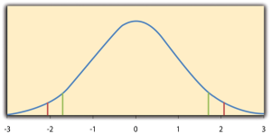
Fortunately, we do not have to deal directly with the distribution of t scores. If we were to enter our sample data and hypothetical mean of interest into one of the online statistical tools in Chapter 12 or into a program like SPSS (Excel does not have a one-sample t- test function), the output would include both the t score and the p value. At this point, the rest of the procedure is simple. If p is equal to or less than .05, we reject the null hypothesis and conclude that the population mean differs from the hypothetical mean of interest. If p is greater than .05, we retain the null hypothesis and conclude that there is not enough evidence to say that the population mean differs from the hypothetical mean of interest. (Again, technically, we conclude only that we do not have enough evidence to conclude that it does differ.)
If we were to compute the t score by hand, we could use a table like Table 13.2 to make the decision. This table does not provide actual p values. Instead, it provides the critical values of t for different degrees of freedom ( df) when α is .05. For now, let us focus on the two-tailed critical values in the last column of the table. Each of these values should be interpreted as a pair of values: one positive and one negative. For example, the two-tailed critical values when there are 24 degrees of freedom are 2.064 and −2.064. These are represented by the red vertical lines in Figure 13.1. The idea is that any t score below the lower critical value (the left-hand red line in Figure 13.1) is in the lowest 2.5% of the distribution, while any t score above the upper critical value (the right-hand red line) is in the highest 2.5% of the distribution. Therefore any t score beyond the critical value in either direction is in the most extreme 5% of t scores when the null hypothesis is true and has a p value less than .05. Thus if the t score we compute is beyond the critical value in either direction, then we reject the null hypothesis. If the t score we compute is between the upper and lower critical values, then we retain the null hypothesis.
Thus far, we have considered what is called a two-tailed test , where we reject the null hypothesis if the t score for the sample is extreme in either direction. This test makes sense when we believe that the sample mean might differ from the hypothetical population mean but we do not have good reason to expect the difference to go in a particular direction. But it is also possible to do a one-tailed test , where we reject the null hypothesis only if the t score for the sample is extreme in one direction that we specify before collecting the data. This test makes sense when we have good reason to expect the sample mean will differ from the hypothetical population mean in a particular direction.
Here is how it works. Each one-tailed critical value in Table 13.2 can again be interpreted as a pair of values: one positive and one negative. A t score below the lower critical value is in the lowest 5% of the distribution, and a t score above the upper critical value is in the highest 5% of the distribution. For 24 degrees of freedom, these values are −1.711 and 1.711. (These are represented by the green vertical lines in Figure 13.1.) However, for a one-tailed test, we must decide before collecting data whether we expect the sample mean to be lower than the hypothetical population mean, in which case we would use only the lower critical value, or we expect the sample mean to be greater than the hypothetical population mean, in which case we would use only the upper critical value. Notice that we still reject the null hypothesis when the t score for our sample is in the most extreme 5% of the t scores we would expect if the null hypothesis were true—so α remains at .05. We have simply redefined extreme to refer only to one tail of the distribution. The advantage of the one-tailed test is that critical values are less extreme. If the sample mean differs from the hypothetical population mean in the expected direction, then we have a better chance of rejecting the null hypothesis. The disadvantage is that if the sample mean differs from the hypothetical population mean in the unexpected direction, then there is no chance at all of rejecting the null hypothesis.
Example One-Sample t – Test
Imagine that a health psychologist is interested in the accuracy of university students’ estimates of the number of calories in a chocolate chip cookie. He shows the cookie to a sample of 10 students and asks each one to estimate the number of calories in it. Because the actual number of calories in the cookie is 250, this is the hypothetical population mean of interest (µ 0 ). The null hypothesis is that the mean estimate for the population (μ) is 250. Because he has no real sense of whether the students will underestimate or overestimate the number of calories, he decides to do a two-tailed test. Now imagine further that the participants’ actual estimates are as follows:
250, 280, 200, 150, 175, 200, 200, 220, 180, 250.
The mean estimate for the sample ( M ) is 212.00 calories and the standard deviation ( SD ) is 39.17. The health psychologist can now compute the t score for his sample:
[latex]t=\dfrac{{212-250}}{\left(\dfrac{39.17}{\sqrt10}\right)}=-3.07[/latex]
If he enters the data into one of the online analysis tools or uses SPSS, it would also tell him that the two-tailed p value for this t score (with 10 − 1 = 9 degrees of freedom) is .013. Because this is less than .05, the health psychologist would reject the null hypothesis and conclude that university students tend to underestimate the number of calories in a chocolate chip cookie. If he computes the t score by hand, he could look at Table 13.2 and see that the critical value of t for a two-tailed test with 9 degrees of freedom is ±2.262. The fact that his t score was more extreme than this critical value would tell him that his p value is less than .05 and that he should reject the null hypothesis. Using APA style, these results would be reported as follows: t (9) = -3.07, p = .01. Note that the t and p are italicized, the degrees of freedom appear in brackets with no decimal remainder, and the values of t and p are rounded to two decimal places.
Finally, if this researcher had gone into this study with good reason to expect that university students underestimate the number of calories, then he could have done a one-tailed test instead of a two-tailed test. The only thing this decision would change is the critical value, which would be −1.833. This slightly less extreme value would make it a bit easier to reject the null hypothesis. However, if it turned out that university students overestimate the number of calories—no matter how much they overestimate it—the researcher would not have been able to reject the null hypothesis.
The Dependent-Samples t – Test
The dependent-samples t -test (sometimes called the paired-samples t- test) is used to compare two means for the same sample tested at two different times or under two different conditions. This comparison is appropriate for pretest-posttest designs or within-subjects experiments. The null hypothesis is that the means at the two times or under the two conditions are the same in the population. The alternative hypothesis is that they are not the same. This test can also be one-tailed if the researcher has good reason to expect the difference goes in a particular direction.
It helps to think of the dependent-samples t- test as a special case of the one-sample t- test. However, the first step in the dependent-samples t- test is to reduce the two scores for each participant to a single difference score by taking the difference between them. At this point, the dependent-samples t- test becomes a one-sample t- test on the difference scores. The hypothetical population mean (µ 0 ) of interest is 0 because this is what the mean difference score would be if there were no difference on average between the two times or two conditions. We can now think of the null hypothesis as being that the mean difference score in the population is 0 (µ 0 = 0) and the alternative hypothesis as being that the mean difference score in the population is not 0 (µ 0 ≠ 0).
Example Dependent-Samples t – Test
Imagine that the health psychologist now knows that people tend to underestimate the number of calories in junk food and has developed a short training program to improve their estimates. To test the effectiveness of this program, he conducts a pretest-posttest study in which 10 participants estimate the number of calories in a chocolate chip cookie before the training program and then again afterward. Because he expects the program to increase the participants’ estimates, he decides to do a one-tailed test. Now imagine further that the pretest estimates are
230, 250, 280, 175, 150, 200, 180, 210, 220, 190
and that the posttest estimates (for the same participants in the same order) are
250, 260, 250, 200, 160, 200, 200, 180, 230, 240.
The difference scores, then, are as follows:
20, 10, −30, 25, 10, 0, 20, −30, 10, 50.
Note that it does not matter whether the first set of scores is subtracted from the second or the second from the first as long as it is done the same way for all participants. In this example, it makes sense to subtract the pretest estimates from the posttest estimates so that positive difference scores mean that the estimates went up after the training and negative difference scores mean the estimates went down.
The mean of the difference scores is 8.50 with a standard deviation of 27.27. The health psychologist can now compute the t score for his sample as follows:
[latex]t=\dfrac{{8.5-0}}{\left(\dfrac{27.27}{\sqrt10}\right)}=1.11[/latex]
If he enters the data into one of the online analysis tools or uses Excel or SPSS, it would tell him that the one-tailed p value for this t score (again with 10 − 1 = 9 degrees of freedom) is .148. Because this is greater than .05, he would retain the null hypothesis and conclude that the training program does not significantly increase people’s calorie estimates. If he were to compute the t score by hand, he could look at Table 13.2 and see that the critical value of t for a one-tailed test with 9 degrees of freedom is 1.833. (It is positive this time because he was expecting a positive mean difference score.) The fact that his t score was less extreme than this critical value would tell him that his p value is greater than .05 and that he should fail to reject the null hypothesis.
The Independent-Samples t- Test
The independent-samples t- test is used to compare the means of two separate samples ( M 1 and M 2 ). The two samples might have been tested under different conditions in a between-subjects experiment, or they could be pre-existing groups in a cross-sectional design (e.g., women and men, extraverts and introverts). The null hypothesis is that the means of the two populations are the same: µ 1 = µ 2 . The alternative hypothesis is that they are not the same: µ 1 ≠ µ 2 . Again, the test can be one-tailed if the researcher has good reason to expect the difference goes in a particular direction.
The t statistic here is a bit more complicated because it must take into account two sample means, two standard deviations, and two sample sizes. The formula is as follows:
[latex]t=\dfrac{{M{_1}-M{_2}}}{\sqrt{\dfrac{SD{^2}{_1}}{n{_1}}+\dfrac{SD{^2}{_2}}{n{_2}}}}[/latex]
Notice that this formula includes squared standard deviations (the variances) that appear inside the square root symbol. Also, lowercase n 1 and n 2 refer to the sample sizes in the two groups or condition (as opposed to capital N , which generally refers to the total sample size). The only additional thing to know here is that there are N − 2 degrees of freedom for the independent-samples t- test.
Example Independent-Samples t – Test
Now the health psychologist wants to compare the calorie estimates of people who regularly eat junk food with the estimates of people who rarely eat junk food. He believes the difference could come out in either direction so he decides to conduct a two-tailed test. He collects data from a sample of eight participants who eat junk food regularly and seven participants who rarely eat junk food. The data are as follows:
Junk food eaters: 180, 220, 150, 85, 200, 170, 150, 190
Non–junk food eaters: 200, 240, 190, 175, 200, 300, 240
The mean for the non-junk food eaters is 220.71 with a standard deviation of 41.23. The mean for the junk food eaters is 168.12 with a standard deviation of 42.66. He can now compute his t score as follows:
[latex]t=\dfrac{{220.71-168.12}}{\sqrt{\dfrac{41.23{^2}}{8}+\dfrac{42.66{^2}}{7}}}= 2.42[/latex]
If he enters the data into one of the online analysis tools or uses Excel or SPSS, it would tell him that the two-tailed p value for this t score (with 15 − 2 = 13 degrees of freedom) is .015. Because this p value is less than .05, the health psychologist would reject the null hypothesis and conclude that people who eat junk food regularly make lower calorie estimates than people who eat it rarely. If he were to compute the t score by hand, he could look at Table 13.2 and see that the critical value of t for a two-tailed test with 13 degrees of freedom is ±2.160. The fact that his t score was more extreme than this critical value would tell him that his p value is less than .05 and that he should reject the null hypothesis.
The Analysis of Variance
T -tests are used to compare two means (a sample mean with a population mean, the means of two conditions or two groups). When there are more than two groups or condition means to be compared, the most common null hypothesis test is the analysis of variance (ANOVA) . In this section, we look primarily at the one-way ANOVA , which is used for between-subjects designs with a single independent variable. We then briefly consider some other versions of the ANOVA that are used for within-subjects and factorial research designs.
One-Way ANOVA
The one-way ANOVA is used to compare the means of more than two samples ( M 1 , M 2 … M G ) in a between-subjects design. The null hypothesis is that all the means are equal in the population: µ 1 = µ 2 =…= µ G . The alternative hypothesis is that not all the means in the population are equal.
The test statistic for the ANOVA is called F . It is a ratio of two estimates of the population variance based on the sample data. One estimate of the population variance is called the mean squares between groups (MS B ) and is based on the differences among the sample means. The other is called the mean squares within groups (MS W ) and is based on the differences among the scores within each group. The F statistic is the ratio of the MS B to the MS W and can, therefore, be expressed as follows:
F = MS B / MS W
Again, the reason that F is useful is that we know how it is distributed when the null hypothesis is true. As shown in Figure 13.2, this distribution is unimodal and positively skewed with values that cluster around 1. The precise shape of the distribution depends on both the number of groups and the sample size, and there are degrees of freedom values associated with each of these. The between-groups degrees of freedom is the number of groups minus one: df B = ( G − 1). The within-groups degrees of freedom is the total sample size minus the number of groups: df W = N − G . Again, knowing the distribution of F when the null hypothesis is true allows us to find the p value.
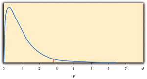
The online tools in Chapter 12 and statistical software such as Excel and SPSS will compute F and find the p value. If p is equal to or less than .05, then we reject the null hypothesis and conclude that there are differences among the group means in the population. If p is greater than .05, then we retain the null hypothesis and conclude that there is not enough evidence to say that there are differences. In the unlikely event that we would compute F by hand, we can use a table of critical values like Table 13.3 “Table of Critical Values of ” to make the decision. The idea is that any F ratio greater than the critical value has a p value of less than .05. Thus if the F ratio we compute is beyond the critical value, then we reject the null hypothesis. If the F ratio we compute is less than the critical value, then we retain the null hypothesis.
Example One-Way ANOVA
Imagine that the health psychologist wants to compare the calorie estimates of psychology majors, nutrition majors, and professional dieticians. He collects the following data:
Psych majors: 200, 180, 220, 160, 150, 200, 190, 200
Nutrition majors: 190, 220, 200, 230, 160, 150, 200, 210, 195
Dieticians: 220, 250, 240, 275, 250, 230, 200, 240
The means are 187.50 ( SD = 23.14), 195.00 ( SD = 27.77), and 238.13 ( SD = 22.35), respectively. So it appears that dieticians made substantially more accurate estimates on average. The researcher would almost certainly enter these data into a program such as Excel or SPSS, which would compute F for him or her and find the p value. Table 13.4 shows the output of the one-way ANOVA function in Excel for these data. This table is referred to as an ANOVA table. It shows that MS B is 5,971.88, MS W is 602.23, and their ratio, F , is 9.92. The p value is .0009. Because this value is below .05, the researcher would reject the null hypothesis and conclude that the mean calorie estimates for the three groups are not the same in the population. Notice that the ANOVA table also includes the “sum of squares” ( SS ) for between groups and for within groups. These values are computed on the way to finding MS B and MS W but are not typically reported by the researcher. Finally, if the researcher were to compute the F ratio by hand, he could look at Table 13.3 and see that the critical value of F with 2 and 21 degrees of freedom is 3.467 (the same value in Table 13.4 under F crit ). The fact that his F score was more extreme than this critical value would tell him that his p value is less than .05 and that he should reject the null hypothesis.
ANOVA Elaborations
Post hoc comparisons.
When we reject the null hypothesis in a one-way ANOVA, we conclude that the group means are not all the same in the population. But this can indicate different things. With three groups, it can indicate that all three means are significantly different from each other. Or it can indicate that one of the means is significantly different from the other two, but the other two are not significantly different from each other. It could be, for example, that the mean calorie estimates of psychology majors, nutrition majors, and dieticians are all significantly different from each other. Or it could be that the mean for dieticians is significantly different from the means for psychology and nutrition majors, but the means for psychology and nutrition majors are not significantly different from each other. For this reason, statistically significant one-way ANOVA results are typically followed up with a series of post hoc comparisons of selected pairs of group means to determine which are different from which others.
One approach to post hoc comparisons would be to conduct a series of independent-samples t- tests comparing each group mean to each of the other group means. But there is a problem with this approach. In general, if we conduct a t -test when the null hypothesis is true, we have a 5% chance of mistakenly rejecting the null hypothesis (see Section 13.3 “Additional Considerations” for more on such Type I errors). If we conduct several t- tests when the null hypothesis is true, the chance of mistakenly rejecting at least one null hypothesis increases with each test we conduct. Thus researchers do not usually make post hoc comparisons using standard t- tests because there is too great a chance that they will mistakenly reject at least one null hypothesis. Instead, they use one of several modified t -test procedures—among them the Bonferonni procedure, Fisher’s least significant difference (LSD) test, and Tukey’s honestly significant difference (HSD) test. The details of these approaches are beyond the scope of this book, but it is important to understand their purpose. It is to keep the risk of mistakenly rejecting a true null hypothesis to an acceptable level (close to 5%).
Repeated-Measures ANOVA
Recall that the one-way ANOVA is appropriate for between-subjects designs in which the means being compared come from separate groups of participants. It is not appropriate for within-subjects designs in which the means being compared come from the same participants tested under different conditions or at different times. This requires a slightly different approach, called the repeated-measures ANOVA . The basics of the repeated-measures ANOVA are the same as for the one-way ANOVA. The main difference is that measuring the dependent variable multiple times for each participant allows for a more refined measure of MS W . Imagine, for example, that the dependent variable in a study is a measure of reaction time. Some participants will be faster or slower than others because of stable individual differences in their nervous systems, muscles, and other factors. In a between-subjects design, these stable individual differences would simply add to the variability within the groups and increase the value of MS W (which would, in turn, decrease the value of F). In a within-subjects design, however, these stable individual differences can be measured and subtracted from the value of MS W . This lower value of MS W means a higher value of F and a more sensitive test.
Factorial ANOVA
When more than one independent variable is included in a factorial design, the appropriate approach is the factorial ANOVA . Again, the basics of the factorial ANOVA are the same as for the one-way and repeated-measures ANOVAs. The main difference is that it produces an F ratio and p value for each main effect and for each interaction. Returning to our calorie estimation example, imagine that the health psychologist tests the effect of participant major (psychology vs. nutrition) and food type (cookie vs. hamburger) in a factorial design. A factorial ANOVA would produce separate F ratios and p values for the main effect of major, the main effect of food type, and the interaction between major and food. Appropriate modifications must be made depending on whether the design is between-subjects, within-subjects, or mixed.
Testing Correlation Coefficients
For relationships between quantitative variables, where Pearson’s r (the correlation coefficient) is used to describe the strength of those relationships, the appropriate null hypothesis test is a test of the correlation coefficient. The basic logic is exactly the same as for other null hypothesis tests. In this case, the null hypothesis is that there is no relationship in the population. We can use the Greek lowercase rho (ρ) to represent the relevant parameter: ρ = 0. The alternative hypothesis is that there is a relationship in the population: ρ ≠ 0. As with the t- test, this test can be two-tailed if the researcher has no expectation about the direction of the relationship or one-tailed if the researcher expects the relationship to go in a particular direction.
It is possible to use the correlation coefficient for the sample to compute a t score with N − 2 degrees of freedom and then to proceed as for a t- test. However, because of the way it is computed, the correlation coefficient can also be treated as its own test statistic. The online statistical tools and statistical software such as Excel and SPSS generally compute the correlation coefficient and provide the p value associated with that value. As always, if the p value is equal to or less than .05, we reject the null hypothesis and conclude that there is a relationship between the variables in the population. If the p value is greater than .05, we retain the null hypothesis and conclude that there is not enough evidence to say there is a relationship in the population. If we compute the correlation coefficient by hand, we can use a table like Table 13.5, which shows the critical values of r for various samples sizes when α is .05. A sample value of the correlation coefficient that is more extreme than the critical value is statistically significant.
Example Test of a Correlation Coefficient
Imagine that the health psychologist is interested in the correlation between people’s calorie estimates and their weight. She has no expectation about the direction of the relationship, so she decides to conduct a two-tailed test. She computes the correlation coefficient for a sample of 22 university students and finds that Pearson’s r is −.21. The statistical software she uses tells her that the p value is .348. It is greater than .05, so she retains the null hypothesis and concludes that there is no relationship between people’s calorie estimates and their weight. If she were to compute the correlation coefficient by hand, she could look at Table 13.5 and see that the critical value for 22 − 2 = 20 degrees of freedom is .444. The fact that the correlation coefficient for her sample is less extreme than this critical value tells her that the p value is greater than .05 and that she should retain the null hypothesis.
A test that involves looking at the difference between two means.
Used to compare a sample mean (M) with a hypothetical population mean (μ0) that provides some interesting standard of comparison.
A statistic (e.g., F , t , etc.) that is computed to compare against what is expected in the null hypothesis, and thus helps find the p value.
The absolute value that a test statistic (e.g., F , t , etc.) must exceed to be considered statistically significant.
Where we reject the null hypothesis if the test statistic for the sample is extreme in either direction (+/-).
Where we reject the null hypothesis only if the t score for the sample is extreme in one direction that we specify before collecting the data.
Used to compare two means for the same sample tested at two different times or under two different conditions (sometimes called the paired-samples t -test).
A method to reduce pairs of scores (e.g., pre- and post-test) to a single score by calculating the difference between them.
Used to compare the means of two separate samples (M1 and M2).
A statistical test used when there are more than two groups or condition means to be compared.
Used for between-subjects designs with a single independent variable.
An estimate of the population variance and is based on the differences among the sample means.
An estimate of the population variance and is based on the differences among the scores within each group.
An unplanned (not hypothesized) test of which pairs of group mean scores are different from which others.
Compares the means from the same participants tested under different conditions or at different times in which the dependent variable is measured multiple times for each participant.
A statistical method to detect differences in the means between conditions when there are two or more independent variables in a factorial design. It allows the detection of main effects and interaction effects.
Research Methods in Psychology Copyright © 2023 by William L. Kelemen, Rajiv S. Jhangiani, I-Chant A. Chiang, Carrie Cuttler, & Dana C. Leighton is licensed under a Creative Commons Attribution-NonCommercial-ShareAlike 4.0 International License , except where otherwise noted.
Share This Book

What is Null Hypothesis? What Is Its Importance in Research?
Scientists begin their research with a hypothesis that a relationship of some kind exists between variables. The null hypothesis is the opposite stating that no such relationship exists. Null hypothesis may seem unexciting, but it is a very important aspect of research. In this article, we discuss what null hypothesis is, how to make use of it, and why you should use it to improve your statistical analyses.
What is the Null Hypothesis?
The null hypothesis can be tested using statistical analysis and is often written as H 0 (read as “H-naught”). Once you determine how likely the sample relationship would be if the H 0 were true, you can run your analysis. Researchers use a significance test to determine the likelihood that the results supporting the H 0 are not due to chance.
The null hypothesis is not the same as an alternative hypothesis. An alternative hypothesis states, that there is a relationship between two variables, while H 0 posits the opposite. Let us consider the following example.
A researcher wants to discover the relationship between exercise frequency and appetite. She asks:
Q: Does increased exercise frequency lead to increased appetite? Alternative hypothesis: Increased exercise frequency leads to increased appetite. H 0 assumes that there is no relationship between the two variables: Increased exercise frequency does not lead to increased appetite.
Let us look at another example of how to state the null hypothesis:
Q: Does insufficient sleep lead to an increased risk of heart attack among men over age 50? H 0 : The amount of sleep men over age 50 get does not increase their risk of heart attack.
Why is Null Hypothesis Important?
Many scientists often neglect null hypothesis in their testing. As shown in the above examples, H 0 is often assumed to be the opposite of the hypothesis being tested. However, it is good practice to include H 0 and ensure it is carefully worded. To understand why, let us return to our previous example. In this case,
Alternative hypothesis: Getting too little sleep leads to an increased risk of heart attack among men over age 50.
H 0 : The amount of sleep men over age 50 get has no effect on their risk of heart attack.
Note that this H 0 is different than the one in our first example. What if we were to conduct this experiment and find that neither H 0 nor the alternative hypothesis was supported? The experiment would be considered invalid . Take our original H 0 in this case, “the amount of sleep men over age 50 get, does not increase their risk of heart attack”. If this H 0 is found to be untrue, and so is the alternative, we can still consider a third hypothesis. Perhaps getting insufficient sleep actually decreases the risk of a heart attack among men over age 50. Because we have tested H 0 , we have more information that we would not have if we had neglected it.
Do I Really Need to Test It?
The biggest problem with the null hypothesis is that many scientists see accepting it as a failure of the experiment. They consider that they have not proven anything of value. However, as we have learned from the replication crisis , negative results are just as important as positive ones. While they may seem less appealing to publishers, they can tell the scientific community important information about correlations that do or do not exist. In this way, they can drive science forward and prevent the wastage of resources.
Do you test for the null hypothesis? Why or why not? Let us know your thoughts in the comments below.

The following null hypotheses were formulated for this study: Ho1. There are no significant differences in the factors that influence urban gardening when respondents are grouped according to age, sex, household size, social status and average combined monthly income.
Rate this article Cancel Reply
Your email address will not be published.

Enago Academy's Most Popular Articles

- Diversity and Inclusion
Need for Diversifying Academic Curricula: Embracing missing voices and marginalized perspectives
In classrooms worldwide, a single narrative often dominates, leaving many students feeling lost. These stories,…

- Career Corner
- Trending Now
Recognizing the signs: A guide to overcoming academic burnout
As the sun set over the campus, casting long shadows through the library windows, Alex…

Reassessing the Lab Environment to Create an Equitable and Inclusive Space
The pursuit of scientific discovery has long been fueled by diverse minds and perspectives. Yet…

- AI in Academia
- Reporting Research
How to Improve Lab Report Writing: Best practices to follow with and without AI-assistance
Imagine you’re a scientist who just made a ground-breaking discovery! You want to share your…

Achieving Research Excellence: Checklist for good research practices
Academia is built on the foundation of trustworthy and high-quality research, supported by the pillars…
7 Steps of Writing an Excellent Academic Book Chapter
When Your Thesis Advisor Asks You to Quit
Virtual Defense: Top 5 Online Thesis Defense Tips

Sign-up to read more
Subscribe for free to get unrestricted access to all our resources on research writing and academic publishing including:
- 2000+ blog articles
- 50+ Webinars
- 10+ Expert podcasts
- 50+ Infographics
- 10+ Checklists
- Research Guides
We hate spam too. We promise to protect your privacy and never spam you.
I am looking for Editing/ Proofreading services for my manuscript Tentative date of next journal submission:

What should universities' stance be on AI tools in research and academic writing?
Chapter 13: Inferential Statistics
Some basic null hypothesis tests, learning objectives.
- Conduct and interpret one-sample, dependent-samples, and independent-samples t tests.
- Interpret the results of one-way, repeated measures, and factorial ANOVAs.
- Conduct and interpret null hypothesis tests of Pearson’s r .
In this section, we look at several common null hypothesis testing procedures. The emphasis here is on providing enough information to allow you to conduct and interpret the most basic versions. In most cases, the online statistical analysis tools mentioned in Chapter 12 will handle the computations—as will programs such as Microsoft Excel and SPSS.
The t Test
As we have seen throughout this book, many studies in psychology focus on the difference between two means. The most common null hypothesis test for this type of statistical relationship is the t test . In this section, we look at three types of t tests that are used for slightly different research designs: the one-sample t test, the dependent-samples t test, and the independent-samples t test.
One-Sample t Test
The one-sample t test is used to compare a sample mean ( M ) with a hypothetical population mean (μ0) that provides some interesting standard of comparison. The null hypothesis is that the mean for the population (µ) is equal to the hypothetical population mean: μ = μ0. The alternative hypothesis is that the mean for the population is different from the hypothetical population mean: μ ≠ μ0. To decide between these two hypotheses, we need to find the probability of obtaining the sample mean (or one more extreme) if the null hypothesis were true. But finding this p value requires first computing a test statistic called t . (A test statistic is a statistic that is computed only to help find the p value.) The formula for t is as follows:

The reason the t statistic (or any test statistic) is useful is that we know how it is distributed when the null hypothesis is true. As shown in Figure 13.1, this distribution is unimodal and symmetrical, and it has a mean of 0. Its precise shape depends on a statistical concept called the degrees of freedom, which for a one-sample t test is N − 1. (There are 24 degrees of freedom for the distribution shown in Figure 13.1.) The important point is that knowing this distribution makes it possible to find the p value for any t score. Consider, for example, a t score of +1.50 based on a sample of 25. The probability of a t score at least this extreme is given by the proportion of t scores in the distribution that are at least this extreme. For now, let us define extreme as being far from zero in either direction. Thus the p value is the proportion of t scores that are +1.50 or above or that are −1.50 or below—a value that turns out to be .14.

Figure 13.1 Distribution of t Scores (With 24 Degrees of Freedom) When the Null Hypothesis Is True. The red vertical lines represent the two-tailed critical values, and the green vertical lines the one-tailed critical values when α = .05.
Fortunately, we do not have to deal directly with the distribution of t scores. If we were to enter our sample data and hypothetical mean of interest into one of the online statistical tools in Chapter 12 or into a program like SPSS (Excel does not have a one-sample t test function), the output would include both the t score and the p value. At this point, the rest of the procedure is simple. If p is less than .05, we reject the null hypothesis and conclude that the population mean differs from the hypothetical mean of interest. If p is greater than .05, we retain the null hypothesis and conclude that there is not enough evidence to say that the population mean differs from the hypothetical mean of interest. (Again, technically, we conclude only that we do not have enough evidence to conclude that it does differ.)
If we were to compute the t score by hand, we could use a table like Table 13.2 to make the decision. This table does not provide actual p values. Instead, it provides the critical values of t for different degrees of freedom ( df) when α is .05. For now, let us focus on the two-tailed critical values in the last column of the table. Each of these values should be interpreted as a pair of values: one positive and one negative. For example, the two-tailed critical values when there are 24 degrees of freedom are +2.064 and −2.064. These are represented by the red vertical lines in Figure 13.1. The idea is that any t score below the lower critical value (the left-hand red line in Figure 13.1) is in the lowest 2.5% of the distribution, while any t score above the upper critical value (the right-hand red line) is in the highest 2.5% of the distribution. Therefore any t score beyond the critical value in either direction is in the most extreme 5% of t scores when the null hypothesis is true and has a p value less than .05. Thus if the t score we compute is beyond the critical value in either direction, then we reject the null hypothesis. If the t score we compute is between the upper and lower critical values, then we retain the null hypothesis.
Thus far, we have considered what is called a two-tailed test , where we reject the null hypothesis if the t score for the sample is extreme in either direction. This test makes sense when we believe that the sample mean might differ from the hypothetical population mean but we do not have good reason to expect the difference to go in a particular direction. But it is also possible to do a one-tailed test , where we reject the null hypothesis only if the t score for the sample is extreme in one direction that we specify before collecting the data. This test makes sense when we have good reason to expect the sample mean will differ from the hypothetical population mean in a particular direction.
Here is how it works. Each one-tailed critical value in Table 13.2 can again be interpreted as a pair of values: one positive and one negative. A t score below the lower critical value is in the lowest 5% of the distribution, and a t score above the upper critical value is in the highest 5% of the distribution. For 24 degrees of freedom, these values are −1.711 and +1.711. (These are represented by the green vertical lines in Figure 13.1.) However, for a one-tailed test, we must decide before collecting data whether we expect the sample mean to be lower than the hypothetical population mean, in which case we would use only the lower critical value, or we expect the sample mean to be greater than the hypothetical population mean, in which case we would use only the upper critical value. Notice that we still reject the null hypothesis when the t score for our sample is in the most extreme 5% of the t scores we would expect if the null hypothesis were true—so α remains at .05. We have simply redefined extreme to refer only to one tail of the distribution. The advantage of the one-tailed test is that critical values are less extreme. If the sample mean differs from the hypothetical population mean in the expected direction, then we have a better chance of rejecting the null hypothesis. The disadvantage is that if the sample mean differs from the hypothetical population mean in the unexpected direction, then there is no chance at all of rejecting the null hypothesis.
Example One-Sample t Test
Imagine that a health psychologist is interested in the accuracy of university students’ estimates of the number of calories in a chocolate chip cookie. He shows the cookie to a sample of 10 students and asks each one to estimate the number of calories in it. Because the actual number of calories in the cookie is 250, this is the hypothetical population mean of interest (µ 0 ). The null hypothesis is that the mean estimate for the population (μ) is 250. Because he has no real sense of whether the students will underestimate or overestimate the number of calories, he decides to do a two-tailed test. Now imagine further that the participants’ actual estimates are as follows:
250, 280, 200, 150, 175, 200, 200, 220, 180, 250.
The mean estimate for the sample ( M ) is 212.00 calories and the standard deviation ( SD ) is 39.17. The health psychologist can now compute the t score for his sample:

Finally, if this researcher had gone into this study with good reason to expect that university students underestimate the number of calories, then he could have done a one-tailed test instead of a two-tailed test. The only thing this decision would change is the critical value, which would be −1.833. This slightly less extreme value would make it a bit easier to reject the null hypothesis. However, if it turned out that university students overestimate the number of calories—no matter how much they overestimate it—the researcher would not have been able to reject the null hypothesis.
The Dependent-Samples t Test
The dependent-samples t test (sometimes called the paired-samples t test) is used to compare two means for the same sample tested at two different times or under two different conditions. This comparison is appropriate for pretest-posttest designs or within-subjects experiments. The null hypothesis is that the means at the two times or under the two conditions are the same in the population. The alternative hypothesis is that they are not the same. This test can also be one-tailed if the researcher has good reason to expect the difference goes in a particular direction.
It helps to think of the dependent-samples t test as a special case of the one-sample t test. However, the first step in the dependent-samples t test is to reduce the two scores for each participant to a single difference score by taking the difference between them. At this point, the dependent-samples t test becomes a one-sample t test on the difference scores. The hypothetical population mean (µ 0 ) of interest is 0 because this is what the mean difference score would be if there were no difference on average between the two times or two conditions. We can now think of the null hypothesis as being that the mean difference score in the population is 0 (µ 0 = 0) and the alternative hypothesis as being that the mean difference score in the population is not 0 (µ 0 ≠ 0).
Example Dependent-Samples t Test
Imagine that the health psychologist now knows that people tend to underestimate the number of calories in junk food and has developed a short training program to improve their estimates. To test the effectiveness of this program, he conducts a pretest-posttest study in which 10 participants estimate the number of calories in a chocolate chip cookie before the training program and then again afterward. Because he expects the program to increase the participants’ estimates, he decides to do a one-tailed test. Now imagine further that the pretest estimates are
230, 250, 280, 175, 150, 200, 180, 210, 220, 190
and that the posttest estimates (for the same participants in the same order) are
250, 260, 250, 200, 160, 200, 200, 180, 230, 240.
The difference scores, then, are as follows:
+20, +10, −30, +25, +10, 0, +20, −30, +10, +50.
Note that it does not matter whether the first set of scores is subtracted from the second or the second from the first as long as it is done the same way for all participants. In this example, it makes sense to subtract the pretest estimates from the posttest estimates so that positive difference scores mean that the estimates went up after the training and negative difference scores mean the estimates went down.
The mean of the difference scores is 8.50 with a standard deviation of 27.27. The health psychologist can now compute the t score for his sample as follows:

The Independent-Samples t Test
The independent-samples t test is used to compare the means of two separate samples ( M 1 and M 2 ). The two samples might have been tested under different conditions in a between-subjects experiment, or they could be preexisting groups in a correlational design (e.g., women and men, extraverts and introverts). The null hypothesis is that the means of the two populations are the same: µ 1 = µ 2 . The alternative hypothesis is that they are not the same: µ 1 ≠ µ 2 . Again, the test can be one-tailed if the researcher has good reason to expect the difference goes in a particular direction.
The t statistic here is a bit more complicated because it must take into account two sample means, two standard deviations, and two sample sizes. The formula is as follows:

Example Independent-Samples t Test
Now the health psychologist wants to compare the calorie estimates of people who regularly eat junk food with the estimates of people who rarely eat junk food. He believes the difference could come out in either direction so he decides to conduct a two-tailed test. He collects data from a sample of eight participants who eat junk food regularly and seven participants who rarely eat junk food. The data are as follows:
Junk food eaters: 180, 220, 150, 85, 200, 170, 150, 190
Non–junk food eaters: 200, 240, 190, 175, 200, 300, 240
The mean for the junk food eaters is 220.71 with a standard deviation of 41.23. The mean for the non–junk food eaters is 168.12 with a standard deviation of 42.66. He can now compute his t score as follows:

The Analysis of Variance
When there are more than two groups or condition means to be compared, the most common null hypothesis test is the analysis of variance (ANOVA) . In this section, we look primarily at the one-way ANOVA , which is used for between-subjects designs with a single independent variable. We then briefly consider some other versions of the ANOVA that are used for within-subjects and factorial research designs.
One-Way ANOVA
The one-way ANOVA is used to compare the means of more than two samples ( M1 , M 2 … M G ) in a between-subjects design. The null hypothesis is that all the means are equal in the population: µ 1 = µ 2 =…= µ G . The alternative hypothesis is that not all the means in the population are equal.
The test statistic for the ANOVA is called F . It is a ratio of two estimates of the population variance based on the sample data. One estimate of the population variance is called the mean squares between groups (MS B ) and is based on the differences among the sample means. The other is called the mean squares within groups (MS W ) and is based on the differences among the scores within each group. The F statistic is the ratio of the MS B to the MS W and can therefore be expressed as follows:
F = MS B / MS W
Again, the reason that F is useful is that we know how it is distributed when the null hypothesis is true. As shown in Figure 13.2, this distribution is unimodal and positively skewed with values that cluster around 1. The precise shape of the distribution depends on both the number of groups and the sample size, and there is a degrees of freedom value associated with each of these. The between-groups degrees of freedom is the number of groups minus one: df B = ( G − 1). The within-groups degrees of freedom is the total sample size minus the number of groups: df W = N − G . Again, knowing the distribution of F when the null hypothesis is true allows us to find the p value.

Figure 13.2 Distribution of the F Ratio With 2 and 37 Degrees of Freedom When the Null Hypothesis Is True. The red vertical line represents the critical value when α is .05.
The online tools in Chapter 12 and statistical software such as Excel and SPSS will compute F and find the p value. If p is less than .05, then we reject the null hypothesis and conclude that there are differences among the group means in the population. If p is greater than .05, then we retain the null hypothesis and conclude that there is not enough evidence to say that there are differences. In the unlikely event that we would compute F by hand, we can use a table of critical values like Table 13.3 “Table of Critical Values of ” to make the decision. The idea is that any F ratio greater than the critical value has a p value of less than .05. Thus if the F ratio we compute is beyond the critical value, then we reject the null hypothesis. If the F ratio we compute is less than the critical value, then we retain the null hypothesis.
Example One-Way ANOVA
Imagine that the health psychologist wants to compare the calorie estimates of psychology majors, nutrition majors, and professional dieticians. He collects the following data:
Psych majors: 200, 180, 220, 160, 150, 200, 190, 200
Nutrition majors: 190, 220, 200, 230, 160, 150, 200, 210, 195
Dieticians: 220, 250, 240, 275, 250, 230, 200, 240
The means are 187.50 ( SD = 23.14), 195.00 ( SD = 27.77), and 238.13 ( SD = 22.35), respectively. So it appears that dieticians made substantially more accurate estimates on average. The researcher would almost certainly enter these data into a program such as Excel or SPSS, which would compute F for him and find the p value. Table 13.4 shows the output of the one-way ANOVA function in Excel for these data. This table is referred to as an ANOVA table. It shows that MS B is 5,971.88, MS W is 602.23, and their ratio, F , is 9.92. The p value is .0009. Because this value is below .05, the researcher would reject the null hypothesis and conclude that the mean calorie estimates for the three groups are not the same in the population. Notice that the ANOVA table also includes the “sum of squares” ( SS ) for between groups and for within groups. These values are computed on the way to finding MS B and MS W but are not typically reported by the researcher. Finally, if the researcher were to compute the F ratio by hand, he could look at Table 13.3 and see that the critical value of F with 2 and 21 degrees of freedom is 3.467 (the same value in Table 13.4 under F crit ). The fact that his F score was more extreme than this critical value would tell him that his p value is less than .05 and that he should reject the null hypothesis.
ANOVA Elaborations
Post hoc comparisons.
When we reject the null hypothesis in a one-way ANOVA, we conclude that the group means are not all the same in the population. But this can indicate different things. With three groups, it can indicate that all three means are significantly different from each other. Or it can indicate that one of the means is significantly different from the other two, but the other two are not significantly different from each other. It could be, for example, that the mean calorie estimates of psychology majors, nutrition majors, and dieticians are all significantly different from each other. Or it could be that the mean for dieticians is significantly different from the means for psychology and nutrition majors, but the means for psychology and nutrition majors are not significantly different from each other. For this reason, statistically significant one-way ANOVA results are typically followed up with a series of post hoc comparisons of selected pairs of group means to determine which are different from which others.
One approach to post hoc comparisons would be to conduct a series of independent-samples t tests comparing each group mean to each of the other group means. But there is a problem with this approach. In general, if we conduct a t test when the null hypothesis is true, we have a 5% chance of mistakenly rejecting the null hypothesis (see Section 13.3 “Additional Considerations” for more on such Type I errors). If we conduct several t tests when the null hypothesis is true, the chance of mistakenly rejecting at least one null hypothesis increases with each test we conduct. Thus researchers do not usually make post hoc comparisons using standard t tests because there is too great a chance that they will mistakenly reject at least one null hypothesis. Instead, they use one of several modified t test procedures—among them the Bonferonni procedure, Fisher’s least significant difference (LSD) test, and Tukey’s honestly significant difference (HSD) test. The details of these approaches are beyond the scope of this book, but it is important to understand their purpose. It is to keep the risk of mistakenly rejecting a true null hypothesis to an acceptable level (close to 5%).
Repeated-Measures ANOVA
Recall that the one-way ANOVA is appropriate for between-subjects designs in which the means being compared come from separate groups of participants. It is not appropriate for within-subjects designs in which the means being compared come from the same participants tested under different conditions or at different times. This requires a slightly different approach, called the repeated-measures ANOVA . The basics of the repeated-measures ANOVA are the same as for the one-way ANOVA. The main difference is that measuring the dependent variable multiple times for each participant allows for a more refined measure of MS W . Imagine, for example, that the dependent variable in a study is a measure of reaction time. Some participants will be faster or slower than others because of stable individual differences in their nervous systems, muscles, and other factors. In a between-subjects design, these stable individual differences would simply add to the variability within the groups and increase the value of MS W . In a within-subjects design, however, these stable individual differences can be measured and subtracted from the value of MS W . This lower value of MS W means a higher value of F and a more sensitive test.
Factorial ANOVA
When more than one independent variable is included in a factorial design, the appropriate approach is the factorial ANOVA . Again, the basics of the factorial ANOVA are the same as for the one-way and repeated-measures ANOVAs. The main difference is that it produces an F ratio and p value for each main effect and for each interaction. Returning to our calorie estimation example, imagine that the health psychologist tests the effect of participant major (psychology vs. nutrition) and food type (cookie vs. hamburger) in a factorial design. A factorial ANOVA would produce separate F ratios and p values for the main effect of major, the main effect of food type, and the interaction between major and food. Appropriate modifications must be made depending on whether the design is between subjects, within subjects, or mixed.
Testing Pearson’s r
For relationships between quantitative variables, where Pearson’s r is used to describe the strength of those relationships, the appropriate null hypothesis test is a test of Pearson’s r . The basic logic is exactly the same as for other null hypothesis tests. In this case, the null hypothesis is that there is no relationship in the population. We can use the Greek lowercase rho (ρ) to represent the relevant parameter: ρ = 0. The alternative hypothesis is that there is a relationship in the population: ρ ≠ 0. As with the t test, this test can be two-tailed if the researcher has no expectation about the direction of the relationship or one-tailed if the researcher expects the relationship to go in a particular direction.
It is possible to use Pearson’s r for the sample to compute a t score with N − 2 degrees of freedom and then to proceed as for a t test. However, because of the way it is computed, Pearson’s r can also be treated as its own test statistic. The online statistical tools and statistical software such as Excel and SPSS generally compute Pearson’s r and provide the p value associated with that value of Pearson’s r . As always, if the p value is less than .05, we reject the null hypothesis and conclude that there is a relationship between the variables in the population. If the p value is greater than .05, we retain the null hypothesis and conclude that there is not enough evidence to say there is a relationship in the population. If we compute Pearson’s r by hand, we can use a table like Table 13.5, which shows the critical values of r for various samples sizes when α is .05. A sample value of Pearson’s r that is more extreme than the critical value is statistically significant.
Example Test of Pearson’s r
Imagine that the health psychologist is interested in the correlation between people’s calorie estimates and their weight. He has no expectation about the direction of the relationship, so he decides to conduct a two-tailed test. He computes the correlation for a sample of 22 university students and finds that Pearson’s r is −.21. The statistical software he uses tells him that the p value is .348. It is greater than .05, so he retains the null hypothesis and concludes that there is no relationship between people’s calorie estimates and their weight. If he were to compute Pearson’s r by hand, he could look at Table 13.5 and see that the critical value for 22 − 2 = 20 degrees of freedom is .444. The fact that Pearson’s r for the sample is less extreme than this critical value tells him that the p value is greater than .05 and that he should retain the null hypothesis.
Key Takeaways
- To compare two means, the most common null hypothesis test is the t test. The one-sample t test is used for comparing one sample mean with a hypothetical population mean of interest, the dependent-samples t test is used to compare two means in a within-subjects design, and the independent-samples t test is used to compare two means in a between-subjects design.
- To compare more than two means, the most common null hypothesis test is the analysis of variance (ANOVA). The one-way ANOVA is used for between-subjects designs with one independent variable, the repeated-measures ANOVA is used for within-subjects designs, and the factorial ANOVA is used for factorial designs.
- A null hypothesis test of Pearson’s r is used to compare a sample value of Pearson’s r with a hypothetical population value of 0.
- Practice: Use one of the online tools, Excel, or SPSS to reproduce the one-sample t test, dependent-samples t test, independent-samples t test, and one-way ANOVA for the four sets of calorie estimation data presented in this section.
- Practice: A sample of 25 university students rated their friendliness on a scale of 1 ( Much Lower Than Average ) to 7 ( Much Higher Than Average ). Their mean rating was 5.30 with a standard deviation of 1.50. Conduct a one-sample t test comparing their mean rating with a hypothetical mean rating of 4 ( Average ). The question is whether university students have a tendency to rate themselves as friendlier than average.
- The correlation between height and IQ is +.13 in a sample of 35.
- For a sample of 88 university students, the correlation between how disgusted they felt and the harshness of their moral judgments was +.23.
- The correlation between the number of daily hassles and positive mood is −.43 for a sample of 30 middle-aged adults.
- Research Methods in Psychology. Authored by : Paul C. Price, Rajiv S. Jhangiani, and I-Chant A. Chiang. Provided by : BCCampus. Located at : https://opentextbc.ca/researchmethods/ . License : CC BY-NC-SA: Attribution-NonCommercial-ShareAlike

Privacy Policy
13.2 Some Basic Null Hypothesis Tests
Learning objectives.
- Conduct and interpret one-sample, dependent-samples, and independent-samples t- tests.
- Interpret the results of one-way, repeated measures, and factorial ANOVAs.
- Conduct and interpret null hypothesis tests of Pearson’s r .
In this section, we look at several common null hypothesis testing procedures. The emphasis here is on providing enough information to allow you to conduct and interpret the most basic versions. In most cases, the online statistical analysis tools mentioned in Chapter 12 will handle the computations—as will programs such as Microsoft Excel and SPSS.
The t- Test
As we have seen throughout this book, many studies in psychology focus on the difference between two means. The most common null hypothesis test for this type of statistical relationship is the t- test . In this section, we look at three types of t tests that are used for slightly different research designs: the one-sample t- test, the dependent-samples t- test, and the independent-samples t- test.
One-Sample t- Test
The one-sample t- test is used to compare a sample mean ( M ) with a hypothetical population mean (μ 0 ) that provides some interesting standard of comparison. The null hypothesis is that the mean for the population (µ) is equal to the hypothetical population mean: μ = μ 0 . The alternative hypothesis is that the mean for the population is different from the hypothetical population mean: μ ≠ μ 0 . To decide between these two hypotheses, we need to find the probability of obtaining the sample mean (or one more extreme) if the null hypothesis were true. But finding this p value requires first computing a test statistic called t . (A test statistic is a statistic that is computed only to help find the p value.) The formula for t is as follows:

The reason the t statistic (or any test statistic) is useful is that we know how it is distributed when the null hypothesis is true. As shown in Figure 13.1, this distribution is unimodal and symmetrical, and it has a mean of 0. Its precise shape depends on a statistical concept called the degrees of freedom, which for a one-sample t -test is N − 1. (There are 24 degrees of freedom for the distribution shown in Figure 13.1.) The important point is that knowing this distribution makes it possible to find the p value for any t score. Consider, for example, a t score of +1.50 based on a sample of 25. The probability of a t score at least this extreme is given by the proportion of t scores in the distribution that are at least this extreme. For now, let us define extreme as being far from zero in either direction. Thus the p value is the proportion of t scores that are +1.50 or above or that are −1.50 or below—a value that turns out to be .14.

Figure 13.1 Distribution of t Scores (With 24 Degrees of Freedom) When the Null Hypothesis Is True. The red vertical lines represent the two-tailed critical values, and the green vertical lines the one-tailed critical values when α = .05.
Fortunately, we do not have to deal directly with the distribution of t scores. If we were to enter our sample data and hypothetical mean of interest into one of the online statistical tools in Chapter 12 or into a program like SPSS (Excel does not have a one-sample t- test function), the output would include both the t score and the p value. At this point, the rest of the procedure is simple. If p is equal to or less than .05, we reject the null hypothesis and conclude that the population mean differs from the hypothetical mean of interest. If p is greater than .05, we retain the null hypothesis and conclude that there is not enough evidence to say that the population mean differs from the hypothetical mean of interest. (Again, technically, we conclude only that we do not have enough evidence to conclude that it does differ.)
If we were to compute the t score by hand, we could use a table like Table 13.2 to make the decision. This table does not provide actual p values. Instead, it provides the critical values of t for different degrees of freedom ( df) when α is .05. For now, let us focus on the two-tailed critical values in the last column of the table. Each of these values should be interpreted as a pair of values: one positive and one negative. For example, the two-tailed critical values when there are 24 degrees of freedom are +2.064 and −2.064. These are represented by the red vertical lines in Figure 13.1. The idea is that any t score below the lower critical value (the left-hand red line in Figure 13.1) is in the lowest 2.5% of the distribution, while any t score above the upper critical value (the right-hand red line) is in the highest 2.5% of the distribution. Therefore any t score beyond the critical value in either direction is in the most extreme 5% of t scores when the null hypothesis is true and has a p value less than .05. Thus if the t score we compute is beyond the critical value in either direction, then we reject the null hypothesis. If the t score we compute is between the upper and lower critical values, then we retain the null hypothesis.
Thus far, we have considered what is called a two-tailed test , where we reject the null hypothesis if the t score for the sample is extreme in either direction. This test makes sense when we believe that the sample mean might differ from the hypothetical population mean but we do not have good reason to expect the difference to go in a particular direction. But it is also possible to do a one-tailed test , where we reject the null hypothesis only if the t score for the sample is extreme in one direction that we specify before collecting the data. This test makes sense when we have good reason to expect the sample mean will differ from the hypothetical population mean in a particular direction.
Here is how it works. Each one-tailed critical value in Table 13.2 can again be interpreted as a pair of values: one positive and one negative. A t score below the lower critical value is in the lowest 5% of the distribution, and a t score above the upper critical value is in the highest 5% of the distribution. For 24 degrees of freedom, these values are −1.711 and +1.711. (These are represented by the green vertical lines in Figure 13.1.) However, for a one-tailed test, we must decide before collecting data whether we expect the sample mean to be lower than the hypothetical population mean, in which case we would use only the lower critical value, or we expect the sample mean to be greater than the hypothetical population mean, in which case we would use only the upper critical value. Notice that we still reject the null hypothesis when the t score for our sample is in the most extreme 5% of the t scores we would expect if the null hypothesis were true—so α remains at .05. We have simply redefined extreme to refer only to one tail of the distribution. The advantage of the one-tailed test is that critical values are less extreme. If the sample mean differs from the hypothetical population mean in the expected direction, then we have a better chance of rejecting the null hypothesis. The disadvantage is that if the sample mean differs from the hypothetical population mean in the unexpected direction, then there is no chance at all of rejecting the null hypothesis.
Example One-Sample t – Test
Imagine that a health psychologist is interested in the accuracy of university students’ estimates of the number of calories in a chocolate chip cookie. He shows the cookie to a sample of 10 students and asks each one to estimate the number of calories in it. Because the actual number of calories in the cookie is 250, this is the hypothetical population mean of interest (µ 0 ). The null hypothesis is that the mean estimate for the population (μ) is 250. Because he has no real sense of whether the students will underestimate or overestimate the number of calories, he decides to do a two-tailed test. Now imagine further that the participants’ actual estimates are as follows:
250, 280, 200, 150, 175, 200, 200, 220, 180, 250.
The mean estimate for the sample ( M ) is 212.00 calories and the standard deviation ( SD ) is 39.17. The health psychologist can now compute the t score for his sample:

Finally, if this researcher had gone into this study with good reason to expect that university students underestimate the number of calories, then he could have done a one-tailed test instead of a two-tailed test. The only thing this decision would change is the critical value, which would be −1.833. This slightly less extreme value would make it a bit easier to reject the null hypothesis. However, if it turned out that university students overestimate the number of calories—no matter how much they overestimate it—the researcher would not have been able to reject the null hypothesis.
The Dependent-Samples t – Test
The dependent-samples t -test (sometimes called the paired-samples t- test) is used to compare two means for the same sample tested at two different times or under two different conditions. This comparison is appropriate for pretest-posttest designs or within-subjects experiments. The null hypothesis is that the means at the two times or under the two conditions are the same in the population. The alternative hypothesis is that they are not the same. This test can also be one-tailed if the researcher has good reason to expect the difference goes in a particular direction.
It helps to think of the dependent-samples t- test as a special case of the one-sample t- test. However, the first step in the dependent-samples t- test is to reduce the two scores for each participant to a single difference score by taking the difference between them. At this point, the dependent-samples t- test becomes a one-sample t- test on the difference scores. The hypothetical population mean (µ 0 ) of interest is 0 because this is what the mean difference score would be if there were no difference on average between the two times or two conditions. We can now think of the null hypothesis as being that the mean difference score in the population is 0 (µ 0 = 0) and the alternative hypothesis as being that the mean difference score in the population is not 0 (µ 0 ≠ 0).
Example Dependent-Samples t – Test
Imagine that the health psychologist now knows that people tend to underestimate the number of calories in junk food and has developed a short training program to improve their estimates. To test the effectiveness of this program, he conducts a pretest-posttest study in which 10 participants estimate the number of calories in a chocolate chip cookie before the training program and then again afterward. Because he expects the program to increase the participants’ estimates, he decides to do a one-tailed test. Now imagine further that the pretest estimates are
230, 250, 280, 175, 150, 200, 180, 210, 220, 190
and that the posttest estimates (for the same participants in the same order) are
250, 260, 250, 200, 160, 200, 200, 180, 230, 240.
The difference scores, then, are as follows:
+20, +10, −30, +25, +10, 0, +20, −30, +10, +50.
Note that it does not matter whether the first set of scores is subtracted from the second or the second from the first as long as it is done the same way for all participants. In this example, it makes sense to subtract the pretest estimates from the posttest estimates so that positive difference scores mean that the estimates went up after the training and negative difference scores mean the estimates went down.
The mean of the difference scores is 8.50 with a standard deviation of 27.27. The health psychologist can now compute the t score for his sample as follows:

The Independent-Samples t- Test
The independent-samples t- test is used to compare the means of two separate samples ( M 1 and M 2 ). The two samples might have been tested under different conditions in a between-subjects experiment, or they could be pre-existing groups in a cross-sectional design (e.g., women and men, extraverts and introverts). The null hypothesis is that the means of the two populations are the same: µ 1 = µ 2 . The alternative hypothesis is that they are not the same: µ 1 ≠ µ 2 . Again, the test can be one-tailed if the researcher has good reason to expect the difference goes in a particular direction.
The t statistic here is a bit more complicated because it must take into account two sample means, two standard deviations, and two sample sizes. The formula is as follows:

Example Independent-Samples t – Test
Now the health psychologist wants to compare the calorie estimates of people who regularly eat junk food with the estimates of people who rarely eat junk food. He believes the difference could come out in either direction so he decides to conduct a two-tailed test. He collects data from a sample of eight participants who eat junk food regularly and seven participants who rarely eat junk food. The data are as follows:
Junk food eaters: 180, 220, 150, 85, 200, 170, 150, 190
Non–junk food eaters: 200, 240, 190, 175, 200, 300, 240
The mean for the non-junk food eaters is 220.71 with a standard deviation of 41.23. The mean for the junk food eaters is 168.12 with a standard deviation of 42.66. He can now compute his t score as follows:

The Analysis of Variance
T -tests are used to compare two means (a sample mean with a population mean, the means of two conditions or two groups). When there are more than two groups or condition means to be compared, the most common null hypothesis test is the analysis of variance (ANOVA) . In this section, we look primarily at the one-way ANOVA , which is used for between-subjects designs with a single independent variable. We then briefly consider some other versions of the ANOVA that are used for within-subjects and factorial research designs.
One-Way ANOVA
The one-way ANOVA is used to compare the means of more than two samples ( M 1 , M 2 … M G ) in a between-subjects design. The null hypothesis is that all the means are equal in the population: µ 1 = µ 2 =…= µ G . The alternative hypothesis is that not all the means in the population are equal.
The test statistic for the ANOVA is called F . It is a ratio of two estimates of the population variance based on the sample data. One estimate of the population variance is called the mean squares between groups (MS B ) and is based on the differences among the sample means. The other is called the mean squares within groups (MS W ) and is based on the differences among the scores within each group. The F statistic is the ratio of the MS B to the MS W and can, therefore, be expressed as follows:
F = MS B / MS W
Again, the reason that F is useful is that we know how it is distributed when the null hypothesis is true. As shown in Figure 13.2, this distribution is unimodal and positively skewed with values that cluster around 1. The precise shape of the distribution depends on both the number of groups and the sample size, and there are degrees of freedom values associated with each of these. The between-groups degrees of freedom is the number of groups minus one: df B = ( G − 1). The within-groups degrees of freedom is the total sample size minus the number of groups: df W = N − G . Again, knowing the distribution of F when the null hypothesis is true allows us to find the p value.

Figure 13.2 Distribution of the F Ratio With 2 and 37 Degrees of Freedom When the Null Hypothesis Is True. The red vertical line represents the critical value when α is .05.
The online tools in Chapter 12 and statistical software such as Excel and SPSS will compute F and find the p value. If p is equal to or less than .05, then we reject the null hypothesis and conclude that there are differences among the group means in the population. If p is greater than .05, then we retain the null hypothesis and conclude that there is not enough evidence to say that there are differences. In the unlikely event that we would compute F by hand, we can use a table of critical values like Table 13.3 “Table of Critical Values of ” to make the decision. The idea is that any F ratio greater than the critical value has a p value of less than .05. Thus if the F ratio we compute is beyond the critical value, then we reject the null hypothesis. If the F ratio we compute is less than the critical value, then we retain the null hypothesis.
Example One-Way ANOVA
Imagine that the health psychologist wants to compare the calorie estimates of psychology majors, nutrition majors, and professional dieticians. He collects the following data:
Psych majors: 200, 180, 220, 160, 150, 200, 190, 200
Nutrition majors: 190, 220, 200, 230, 160, 150, 200, 210, 195
Dieticians: 220, 250, 240, 275, 250, 230, 200, 240
The means are 187.50 ( SD = 23.14), 195.00 ( SD = 27.77), and 238.13 ( SD = 22.35), respectively. So it appears that dieticians made substantially more accurate estimates on average. The researcher would almost certainly enter these data into a program such as Excel or SPSS, which would compute F for him or her and find the p value. Table 13.4 shows the output of the one-way ANOVA function in Excel for these data. This table is referred to as an ANOVA table. It shows that MS B is 5,971.88, MS W is 602.23, and their ratio, F , is 9.92. The p value is .0009. Because this value is below .05, the researcher would reject the null hypothesis and conclude that the mean calorie estimates for the three groups are not the same in the population. Notice that the ANOVA table also includes the “sum of squares” ( SS ) for between groups and for within groups. These values are computed on the way to finding MS B and MS W but are not typically reported by the researcher. Finally, if the researcher were to compute the F ratio by hand, he could look at Table 13.3 and see that the critical value of F with 2 and 21 degrees of freedom is 3.467 (the same value in Table 13.4 under F crit ). The fact that his F score was more extreme than this critical value would tell him that his p value is less than .05 and that he should reject the null hypothesis.
ANOVA Elaborations
Post hoc comparisons.
When we reject the null hypothesis in a one-way ANOVA, we conclude that the group means are not all the same in the population. But this can indicate different things. With three groups, it can indicate that all three means are significantly different from each other. Or it can indicate that one of the means is significantly different from the other two, but the other two are not significantly different from each other. It could be, for example, that the mean calorie estimates of psychology majors, nutrition majors, and dieticians are all significantly different from each other. Or it could be that the mean for dieticians is significantly different from the means for psychology and nutrition majors, but the means for psychology and nutrition majors are not significantly different from each other. For this reason, statistically significant one-way ANOVA results are typically followed up with a series of post hoc comparisons of selected pairs of group means to determine which are different from which others.
One approach to post hoc comparisons would be to conduct a series of independent-samples t- tests comparing each group mean to each of the other group means. But there is a problem with this approach. In general, if we conduct a t -test when the null hypothesis is true, we have a 5% chance of mistakenly rejecting the null hypothesis (see Section 13.3 “Additional Considerations” for more on such Type I errors). If we conduct several t- tests when the null hypothesis is true, the chance of mistakenly rejecting at least one null hypothesis increases with each test we conduct. Thus researchers do not usually make post hoc comparisons using standard t- tests because there is too great a chance that they will mistakenly reject at least one null hypothesis. Instead, they use one of several modified t -test procedures—among them the Bonferonni procedure, Fisher’s least significant difference (LSD) test, and Tukey’s honestly significant difference (HSD) test. The details of these approaches are beyond the scope of this book, but it is important to understand their purpose. It is to keep the risk of mistakenly rejecting a true null hypothesis to an acceptable level (close to 5%).
Repeated-Measures ANOVA
Recall that the one-way ANOVA is appropriate for between-subjects designs in which the means being compared come from separate groups of participants. It is not appropriate for within-subjects designs in which the means being compared come from the same participants tested under different conditions or at different times. This requires a slightly different approach, called the repeated-measures ANOVA . The basics of the repeated-measures ANOVA are the same as for the one-way ANOVA. The main difference is that measuring the dependent variable multiple times for each participant allows for a more refined measure of MS W . Imagine, for example, that the dependent variable in a study is a measure of reaction time. Some participants will be faster or slower than others because of stable individual differences in their nervous systems, muscles, and other factors. In a between-subjects design, these stable individual differences would simply add to the variability within the groups and increase the value of MS W (which would, in turn, decrease the value of F). In a within-subjects design, however, these stable individual differences can be measured and subtracted from the value of MS W . This lower value of MS W means a higher value of F and a more sensitive test.
Factorial ANOVA
When more than one independent variable is included in a factorial design, the appropriate approach is the factorial ANOVA . Again, the basics of the factorial ANOVA are the same as for the one-way and repeated-measures ANOVAs. The main difference is that it produces an F ratio and p value for each main effect and for each interaction. Returning to our calorie estimation example, imagine that the health psychologist tests the effect of participant major (psychology vs. nutrition) and food type (cookie vs. hamburger) in a factorial design. A factorial ANOVA would produce separate F ratios and p values for the main effect of major, the main effect of food type, and the interaction between major and food. Appropriate modifications must be made depending on whether the design is between-subjects, within-subjects, or mixed.
Testing Correlation Coefficients
For relationships between quantitative variables, where Pearson’s r (the correlation coefficient) is used to describe the strength of those relationships, the appropriate null hypothesis test is a test of the correlation coefficient. The basic logic is exactly the same as for other null hypothesis tests. In this case, the null hypothesis is that there is no relationship in the population. We can use the Greek lowercase rho (ρ) to represent the relevant parameter: ρ = 0. The alternative hypothesis is that there is a relationship in the population: ρ ≠ 0. As with the t- test, this test can be two-tailed if the researcher has no expectation about the direction of the relationship or one-tailed if the researcher expects the relationship to go in a particular direction.
It is possible to use the correlation coefficient for the sample to compute a t score with N − 2 degrees of freedom and then to proceed as for a t- test. However, because of the way it is computed, the correlation coefficient can also be treated as its own test statistic. The online statistical tools and statistical software such as Excel and SPSS generally compute the correlation coefficient and provide the p value associated with that value. As always, if the p value is equal to or less than .05, we reject the null hypothesis and conclude that there is a relationship between the variables in the population. If the p value is greater than .05, we retain the null hypothesis and conclude that there is not enough evidence to say there is a relationship in the population. If we compute the correlation coefficient by hand, we can use a table like Table 13.5, which shows the critical values of r for various samples sizes when α is .05. A sample value of the correlation coefficient that is more extreme than the critical value is statistically significant.
Example Test of a Correlation Coefficient
Imagine that the health psychologist is interested in the correlation between people’s calorie estimates and their weight. She has no expectation about the direction of the relationship, so she decides to conduct a two-tailed test. She computes the correlation coefficient for a sample of 22 university students and finds that Pearson’s r is −.21. The statistical software she uses tells her that the p value is .348. It is greater than .05, so she retains the null hypothesis and concludes that there is no relationship between people’s calorie estimates and their weight. If she were to compute the correlation coefficient by hand, she could look at Table 13.5 and see that the critical value for 22 − 2 = 20 degrees of freedom is .444. The fact that the correlation coefficient for her sample is less extreme than this critical value tells her that the p value is greater than .05 and that she should retain the null hypothesis.
Key Takeaways
- To compare two means, the most common null hypothesis test is the t- test. The one-sample t- test is used for comparing one sample mean with a hypothetical population mean of interest, the dependent-samples t- test is used to compare two means in a within-subjects design, and the independent-samples t- test is used to compare two means in a between-subjects design.
- To compare more than two means, the most common null hypothesis test is the analysis of variance (ANOVA). The one-way ANOVA is used for between-subjects designs with one independent variable, the repeated-measures ANOVA is used for within-subjects designs, and the factorial ANOVA is used for factorial designs.
- A null hypothesis test of Pearson’s r is used to compare a sample value of Pearson’s r with a hypothetical population value of 0.
- Practice: Use one of the online tools, Excel, or SPSS to reproduce the one-sample t- test, dependent-samples t- test, independent-samples t- test, and one-way ANOVA for the four sets of calorie estimation data presented in this section.
- Practice: A sample of 25 university students rated their friendliness on a scale of 1 ( Much Lower Than Average ) to 7 ( Much Higher Than Average ). Their mean rating was 5.30 with a standard deviation of 1.50. Conduct a one-sample t- test comparing their mean rating with a hypothetical mean rating of 4 ( Average ). The question is whether university students have a tendency to rate themselves as friendlier than average.
- The correlation between height and IQ is +.13 in a sample of 35.
- For a sample of 88 university students, the correlation between how disgusted they felt and the harshness of their moral judgments was +.23.
- The correlation between the number of daily hassles and positive mood is −.43 for a sample of 30 middle-aged adults.

Share This Book
- Increase Font Size
IMAGES
VIDEO
COMMENTS
A crucial step in null hypothesis testing is finding the likelihood of the sample result if the null hypothesis were true. This probability is called the p value. A low p value means that the sample result would be unlikely if the null hypothesis were true and leads to the rejection of the null hypothesis. A high p value means that the sample ...
The null hypothesis (H 0), stated as the null, is a statement about a population parameter, such as the population mean, that is assumed to be true. The null hypothesis is a starting point. We will test whether the value stated in the null hypothesis is likely to be true. Keep in mind that the only reason we are testing the null hypothesis is ...
A crucial step in null hypothesis testing is finding the likelihood of the sample result if the null hypothesis were true. This probability is called the p value. A low p value means that the sample result would be unlikely if the null hypothesis were true and leads to the rejection of the null hypothesis. A p value that is not low means that ...
Null Hypothesis H 0: The correlation in the population is zero: ρ = 0. Alternative Hypothesis H A: The correlation in the population is not zero: ρ ≠ 0. For all these cases, the analysts define the hypotheses before the study. After collecting the data, they perform a hypothesis test to determine whether they can reject the null hypothesis.
The null and alternative hypotheses offer competing answers to your research question. When the research question asks "Does the independent variable affect the dependent variable?": The null hypothesis ( H0) answers "No, there's no effect in the population.". The alternative hypothesis ( Ha) answers "Yes, there is an effect in the ...
illustrates a null hypothesis. Designing Research Example 7.3 A Null Hypothesis An investigator might examine three types of reinforcement for children with autism: verbal cues, a reward, and no reinforcement. The investigator collects behavioral measures assessing social interaction of the children with their siblings. A null hypothesis might ...
In scientific research, the null hypothesis (often denoted H 0) is the claim that the effect being studied does not exist. The null hypothesis can also be described as the hypothesis in which no relationship exists between two sets of data or variables being analyzed. If the null hypothesis is true, any experimentally observed effect is due to ...
This null hypothesis can be written as: H0: X¯ = μ H 0: X ¯ = μ. For most of this textbook, the null hypothesis is that the means of the two groups are similar. Much later, the null hypothesis will be that there is no relationship between the two groups. Either way, remember that a null hypothesis is always saying that nothing is different.
Figure 13.2 Distribution of the F Ratio With 2 and 37 Degrees of Freedom When the Null Hypothesis Is True. The red vertical line represents the critical value when α is .05. The online tools in Chapter 12 "Descriptive Statistics" and statistical software such as Excel and SPSS will compute F and find the p value.
The Logic of Null Hypothesis Testing. Null hypothesis testing (often called null hypothesis significance testing or NHST) is a formal approach to deciding between two interpretations of a statistical relationship in a sample. One interpretation is called the null hypothesis (often symbolized H0 and read as "H-zero").
Review. In a hypothesis test, sample data is evaluated in order to arrive at a decision about some type of claim.If certain conditions about the sample are satisfied, then the claim can be evaluated for a population. In a hypothesis test, we: Evaluate the null hypothesis, typically denoted with \(H_{0}\).The null is not rejected unless the hypothesis test shows otherwise.
A crucial step in null hypothesis testing is finding the likelihood of the sample result if the null hypothesis were true. This probability is called the p value. A low p value means that the sample result would be unlikely if the null hypothesis were true and leads to the rejection of the null hypothesis. A high p value means that the sample ...
INTRODUCTION. Scientific research is usually initiated by posing evidenced-based research questions which are then explicitly restated as hypotheses.1,2 The hypotheses provide directions to guide the study, solutions, explanations, and expected results.3,4 Both research questions and hypotheses are essentially formulated based on conventional theories and real-world processes, which allow the ...
The Logic of Null Hypothesis Testing. Null hypothesis testing (often called null hypothesis significance testing or NHST) is a formal approach to deciding between two interpretations of a statistical relationship in a sample. One interpretation is called the null hypothesis (often symbolized H0 and read as "H-zero").
A crucial step in null hypothesis testing is finding the likelihood of the sample result if the null hypothesis were true. This probability is called the p value. A low p value means that the sample result would be unlikely if the null hypothesis were true and leads to the rejection of the null hypothesis. A p value that is not low means that ...
This chapter lays out the basic logic and process of hypothesis testing. We will perform z tests, which use the z score formula from Chapter 6 and data from a sample mean to make an inference about a population.. Logic and Purpose of Hypothesis Testing. A hypothesis is a prediction that is tested in a research study. The statistician R. A. Fisher explained the concept of hypothesis testing ...
The Logic of Null Hypothesis Testing. Null hypothesis testing (often called null hypothesis significance testing or NHST) is a formal approach to deciding between two interpretations of a statistical relationship in a sample. One interpretation is called the null hypothesis (often symbolized H0 and read as "H-zero").
Uses p-values to point at the absence of an effect or accept the null hypothesis. 11 Does not use p-values to point at the absence of effect or accept the null hypothesis. 29 Not applicable. 3 "Statistical" significance. Does not explicitly refer to "statistical significance" 23 Consistently refers to "statistical significance" 3
The most common null hypothesis test for this type of statistical relationship is the t- test. In this section, we look at three types of t tests that are used for slightly different research designs: the one-sample t- test, the dependent-samples t- test, and the independent-samples t- test. You may have already taken a course in statistics ...
The null hypothesis is the opposite stating that no such relationship exists. Null hypothesis may seem unexciting, but it is a very important aspect of research. In this article, we discuss what null hypothesis is, how to make use of it, and why you should use it to improve your statistical analyses.
The online tools in Chapter 12 and statistical software such as Excel and SPSS will compute F and find the p value. If p is less than .05, then we reject the null hypothesis and conclude that there are differences among the group means in the population.If p is greater than .05, then we retain the null hypothesis and conclude that there is not enough evidence to say that there are differences.
The t-Test. As we have seen throughout this book, many studies in psychology focus on the difference between two means. The most common null hypothesis test for this type of statistical relationship is the t- test. In this section, we look at three types of t tests that are used for slightly different research designs: the one-sample t- test ...