write a short note on life cycle hypothesis

Life-Cycle Hypothesis

Definition: The Life-cycle hypothesis was developed by Franco Modigliani in 1957. The theory states that individuals seek to smooth consumption over the course of a lifetime – borrowing in times of low-income and saving during periods of high income.

• As a student, it is rational to borrow to fund education.
• Then during your working life, you pay off student loans and begin saving for your retirement.
• This saving during working life enables you to maintain similar levels of income during your retirement.

It suggests wealth will build up in working age, but then fall in retirement.

Wealth in the Life-Cycle Hypothesis

The theory states consumption will be a function of wealth, expected lifetime earnings and the number of years until retirement.

Consumption will depend on

• C= consumption
• R = Years until retirement. Remaining years of work
• T= Remaining years of life

It suggests for the whole economy consumption will be a function of both wealth and income.

Prior to life-cycle theories, it was assumed that consumption was a function of income. For example, the Keynesian consumption function saw a more direct link between income and spending.

However, this failed to account for how consumption may vary depending on the position in life-cycle.

Motivation for life-cycle consumption patterns

• Diminishing marginal utility of income. If income is high during working life, there is a diminishing marginal utility of spending extra money at that particular time.
• Harder to work and earn money, in old age. Life Cycle enables people to work hard and spend less.

Does the Life-cycle theory happen in reality?

Mervyn King suggests life-cycle consumption patterns can be found in approx 75% of the population. However, 20-25% don’t plan in the long term. (NBER paper on economics of saving )

Reasons for why people don’t smooth consumption over a lifetime.

• Present focus bias – People can find it hard to value income a long time in the future
• Inertia and status quo bias . Planning for retirement requires effort, forward thinking and knowledge of financial instruments such as pensions. People may prefer to procrastinate – even though they know they should save more – and so saving gets put off.

Criticisms of Life Cycle Theory

• It assumes people run down wealth in old age, but often this doesn’t happen as people would like to pass on inherited wealth to children. Also, there can be an attachment to wealth and an unwillingness to run it down. See: Prospect theory and the endowment effect.
• It assumes people are rational and forward planning. Behavioural economics suggests many people have motivations to avoid planning.
• People may lack the self-control to reduce spending now and save more for future.
• Life-cycle is easier for people on high incomes. They are more likely to have financial knowledge, also they have the ‘luxury’ of being able to save. People on low-incomes, with high credit card debts, may feel there is no disposable income to save.
• Leisure. Rather than smoothing out consumption, individuals may prefer to smooth out leisure – working fewer hours during working age, and continuing to work part-time in retirement.
• Government means-tested benefits for old-age people may provide an incentive not to save because lower savings will lead to more social security payments.

Other theories

• Permanent income hypothesis of Milton Friedman – This states people only spend more when they see it as an increase in permanent income.
• Ricardian Equivalence  – consumers may see tax cuts as only a temporary rise in income so will not alter spending.
• Autonomous consumption – In Keynesian consumption function, the level of consumption that is independent of income.
• Marginal propensity to consume – how much of extra income is spent.

15 thoughts on “Life-Cycle Hypothesis”

Thanks for the reminder of the theory… Am a moi university Economic student in Nairobi Kenya.

Thanks for the most summarised note ever. it will help me with presentation. Gulu university. JALON

prof premraj pushpakaran writes — 2018 marks the 100th birth year of Franco Modigliani!!!

Thanks for the analysis on the hypothesis

Nice piece of work for economist. Been applicable in my presentation at Kyambogo university Uganda

This piece of paper is very important as far as consumption is concerned…

This piece is the best I have seen so far, this is a great work

Thanks for this work.it Will help me in my presentation at metropolitan international University

Very coincise and well articulated. This work reconnects me with themechanics of consumption theories. I appreaciate for a job well done.

Very nice and comprensive information. It will help me in my exams at university of jos Nigeria, studying economics

thank u for the summarized notes,it will help me in my exam at Kibabii university

Great job. Thanks for this masterpiece.

Good job. Thanks for this masterpiece. It reconnects me with the consumption theories.

A good summarised piece of work on life cycle hypothesis, it will help me in my group presentation. Kenyatta University economics student.

Comments are closed.

Quickonomics

Life-Cycle Hypothesis (Lch)

Definition of life-cycle hypothesis (lch).

The Life-Cycle Hypothesis (LCH) is an economic theory that suggests individuals base their consumption and savings decisions on their expected lifetime income rather than their current income. According to the LCH, individuals strive to maintain a stable standard of living throughout their lifetime by adjusting their savings and consumption patterns. This hypothesis takes into account the different stages of life, such as education, working years, and retirement, and assumes individuals plan and save accordingly for these stages.

To illustrate the Life-Cycle Hypothesis, let’s consider two individuals: Alan, a young professional just starting his career, and Sarah, a retiree. Alan expects his income to increase significantly over time as he gains experience and advances in his profession. To maintain a stable standard of living, he saves a portion of his income during his early working years, which allows him to enjoy a more comfortable retirement.

On the other hand, Sarah has already retired and relies on savings and pensions for her income. Since she is no longer earning a salary, her consumption decreases to meet her reduced income. She draws from her accumulated savings to support her lifestyle in retirement.

Throughout their lives, both Alan and Sarah make consumption and savings decisions based on their expected lifetime income, adjusting their behavior accordingly.

Why the Life-Cycle Hypothesis Matters

The Life-Cycle Hypothesis provides a framework for understanding individuals’ consumption and savings patterns over their lifetimes. It emphasizes the importance of long-term financial planning and highlights the trade-off between current consumption and saving for the future.

Understanding the Life-Cycle Hypothesis is useful for policymakers, financial planners, and individuals themselves. Policymakers can design policies and programs that support retirement savings and encourage long-term financial stability. Financial planners can help individuals develop strategies to achieve their desired lifestyles in retirement. Lastly, individuals can benefit from understanding their own consumption patterns and making informed decisions about savings and retirement planning.

To provide the best experiences, we and our partners use technologies like cookies to store and/or access device information. Consenting to these technologies will allow us and our partners to process personal data such as browsing behavior or unique IDs on this site and show (non-) personalized ads. Not consenting or withdrawing consent, may adversely affect certain features and functions.

Click below to consent to the above or make granular choices. Your choices will be applied to this site only. You can change your settings at any time, including withdrawing your consent, by using the toggles on the Cookie Policy, or by clicking on the manage consent button at the bottom of the screen.

• Search Search Please fill out this field.
• Financial Planning

What Is the Life-Cycle Hypothesis?

The Life-Cycle Hypothesis Explained

Definition and Examples of the Life-Cycle Hypothesis

How the life-cycle hypothesis works, criticisms of the life-cycle hypothesis, life-cycle hypothesis theory vs. permanent income hypothesis theory.

Ridofranz / Getty Images

The life-cycle hypothesis (LCH) is an economic theory that suggests that individuals have a tendency to maintain the same level of spending over time. They achieve this goal by borrowing in when they're younger and their income is low, saving during their middle years when income is high, and living off their assets in their older years when income is low again. 

Here’s a closer look at how the LCH works and why it’s important.

The LCH states that households save and spend their wealth in an effort to keep their consumption level steady over time. Even though wealth and income may vary over your lifetime, the theory states, your spending habits stay relatively the same. 

• Acronym: LCH
• Alternate name: Life-cycle model

Saving for retirement is a good example of the LCH in action. You know your income may disappear when you’re older, so you save money during your working years to afford the same lifestyle later on.

The LCH predicts that, in general, you maintain the same level of consumption throughout your lifetime by: 

• Borrowing money when you’re young (either by borrowing money or liquidating assets you already own)
• Saving more money when you’re middle aged and at the peak of your career
• Living off the wealth you’ve accumulated when you’re old and retired 

Franco Modigliani published the life-cycle hypothesis theory in 1954 with Richard Brumberg and later won a Nobel Prize for his economic analyses.

The LCH predicts that your savings habits follow a hump-shaped pattern as in the diagram below where your savings rate is low during your younger and older years and peaks during your middle years:

For example, suppose you make $20,000 this year, but you expect your income will increase to $80,000 next year because you’ve got a job lined up after you graduate from college.

According to the LCH, you may spend money today with your future income in mind, which may lead you to borrow money. As you reach the peak of your career, you’ll pay off any debt you accumulated and ramp up your savings. Then, you’ll draw down that savings in retirement so you can continue your same level of spending.

The LCH has withstood the test of time but it’s not without its flaws: 

LCH Doesn’t Account for Financial Windfalls

Traditional LCH models don’t apply to individuals who run into financial windfalls or have sporadic income throughout their lives. 

Take NFL players, for example. The LCH would imply that NFL players save considerable amounts of money while they’re at the peak of their careers so they can sustain the same level of consumption when they retire. 

But the reality is that some NFL athletes go from enormously wealthy to near poverty shortly after the end of their careers. A 2015 National Bureau of Economic Research study that focused on LCH and the NFL predicted that an NFL player has a 15% to 40% chance of going bankrupt 25 years after they retire. 

The study said the high bankruptcy rates may be due to the fact that players:

• Think their career will last longer than it typically does
• Make poor financial decisions with the money they receive
• Have social pressures to spend more than they should 

LCH Assumes Your Consumption Level Will Stay the Same

The LCH predicts that you’ll maintain roughly your same level of spending by borrowing money when income is low and saving when income is high. But this isn’t always realistic. 

For example, younger workers may not have access to the credit needed to fund their ideal level of spending now. So, naturally, their consumption habits would change as their income increased and those options became available to them. 

Likewise, a family with parents in their 30s with three young kids, student loan debt, and a mortgage may consume more now than they will in their 70s when they’re retired, possibly debt-free, and no longer have dependents to care for.

Both the LCH theory and the permanent income hypothesis (PIH) theory seek to understand how individuals spend and save money. The main difference is that the LCH is based on a finite timeline where a person saves only enough to sustain their spending habits during their lifetime. The PIH, on the other hand, is based on an infinite timeline where a person saves enough for both themselves and their heirs.

Key Takeaways

• The life-cycle hypothesis (LCH) is an economic theory that describes how an individual maintains roughly the same level of consumption over time by saving when their income is high and borrowing when income is low.
• The LCH predicts that wealth accumulation follows a hump-shaped curve where you have a low savings rate when you’re young, a high rate when you’re middle-aged, and a low rate again when you’re old.
• Some experts criticize the LCH because consumption doesn’t always stay consistent over time. For example, a middle-aged worker with three kids and a mortgage probably consumes more than they will when they’re retired with no debt or dependents.

Massachusetts Institute of Technology. " The Collected Papers of Franco Modigliani, Volume 6 ."

Federal Reserve Board. " A Primer on the Economics and Time Series Econometrics of Wealth Effects ," Page 8.

Carnegie Mellon University. " The Life Cycle Theory of Consumption ," Page 340.

National Bureau of Economic Research. " Bankruptcy Rates Among NFL Players With Short-Lived Income Spikes ," Page 8.

Centre for Economic Studies and Finance. " Working Paper No. 140: The Life-Cycle Hypothesis, Fiscal Policy,and Social Security ," Page 7.

Life-cycle hypothesis: Ando and Modigliani

• Post author: Viren Rehal
• Post published: August 18, 2022
• Post category: Consumption function / Macroeconomics
• Post comments: 0 Comments

The life-cycle hypothesis was postulated by Ando and Modigliani in an attempt to explain the behaviour of consumption function in the long and short run. According to this theory, current consumption decisions are based on future expected income over an individual’s lifetime. The major advantage of this theory is that Ando and Modigliani incorporated the role of assets in determining consumption decisions. Other theories don’t incorporate assets into consumption ( absolute income hypothesis ) or the role of assets is only implicit ( permanent income hypothesis ).

MPC < APC in cross-sections

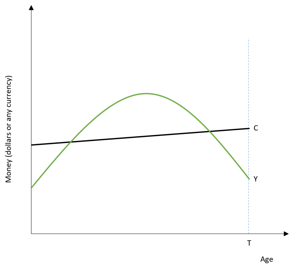
Over the lifetime of any individual, income is low in the early years of life. As people reach middle age, their income rises as they start earning more. In later years of life, however, income starts falling again to reach low levels owing to retirement or the inability to work as people grow older. Therefore, income starts from a low level, keeps increasing in middle age, and declines back to a low level in old age.

In the case of consumption, individuals are expected to maintain a constant or slightly increasing level of consumption as they keep growing older. Since consumption is dependent on future expected income, the present value of consumption is constrained by the present value of income.

APC and MPS at different age

During the early years, income is low as compared to consumption and individuals are borrowers during this period, i.e. APC is high. However, they expect their future income to rise during their middle age. Because income is higher than consumption level, they pay off their borrowings during this period and save for retirement in old age. With high income, APC is low because consumption is much lower as compared to income in this period. In the later years of the life-cycle, income is again below consumption level. Hence, this is a period of dissavings or negative savings by individuals, leading to a low APC.

Therefore, across different sections based on income levels, APC will be high for low-income groups. These low-income groups primarily include people in their early years of life and people in old age, who have low incomes. On average, APC will be high as the low-income group consists of higher than average young and older people. On the contrary, high-income groups will have a higher than average proportion of middle-aged people. This is because they have higher incomes. APC, in this case, will be lower because consumption is low compared to income level during middle age.

Hence, APC will decline as income increases and MPC<APC in cross sections because of different income levels in a life-cycle.

consumption function of Life-Cycle Hypothesis

According to the life-cycle hypothesis, the consumption of any individual is based on expected income in the future. If the expected income rises, the consumption of that consumer will also increase. Ando and Modigliani use the Present Value criterion to represent expected income in the future. Therefore, the consumption of an individual can be expressed as follows:

If the present value of expected income increases, then consumption of that consumer will increase by a given proportion ( theta ) of that increase in income.

If the income distribution and age of the population are stable along with the constant taste and preferences of consumers, then the aggregate consumption function can simply be obtained by summation of all individual consumption functions.

Present Value of expected future income

Future income is unknown and cannot be measured directly. Therefore, the present value of expected income has to be estimated indirectly. Ando and Modigliani divided income into two types- income labour and income from assets, and estimated the present value variable as follows:

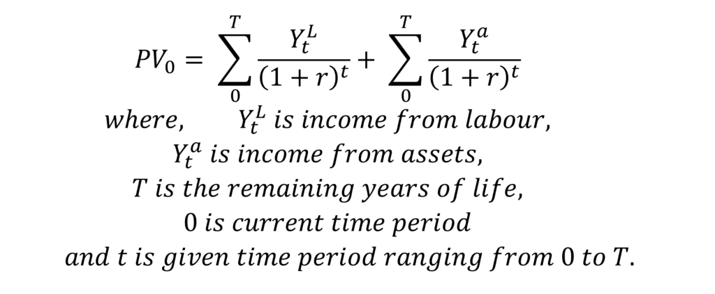
In an efficient capital market, we can assume that the present value of income from assets is equal to the value of assets in the current time period. Therefore, we can substitute the second element of the equation as:

In the case of the first element of income from labour, we know the labour income in the current period and can therefore separate current income from the present value of expected income.

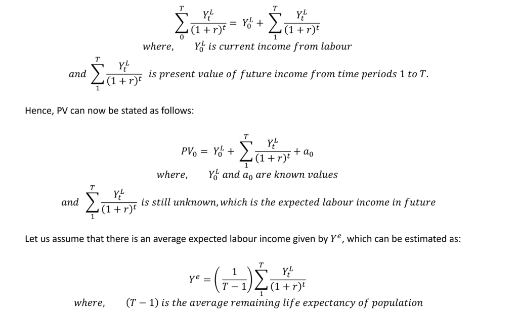
Therefore, the above equation simply divides the expected future labour income by the average life remaining of the population in years to estimate an average expected labour income. From this equation, we have:

In this equation, Y e  is the only unknown which is an estimate of average expected labour income.

Ando and Modigliani found that assuming this average expected labour income as a function of current labour income worked well and they stated this as:

This implies that if current income increases, people expect average future income to rise as well. The amount of this rise is determined by the proportion coefficient (beta), such that an increase in average expected income is a proportion of current labour income.

Hence, we can modify the PV 0  equation and the consumption function as follows:

This equation represents the consumption function associated with the life-cycle hypothesis. Every variable in this equation can be measured which allows empirical estimation of the consumption function.

cyclical fluctuation and long-run consumption: empirical results

The consumption function put forward by Ando and Modigliani can be used to carry out empirical analysis to understand the behaviour of consumption in the long run and the effect of business cycles on consumption.

Ando and Modigliani applied this consumption function to annual data of the United States. They obtained the following results:

The marginal propensity to consume from labour income is 0.7. This means that a $1 increase in labour income will lead to a $0.7 increase in consumption. Similarly, the marginal propensity to consume from assets is 0.06 implying that a $1 increase in assets (net worth of assets) will lead to a $0.06 increase in consumption.

Let us apply these results to the life cycle consumption function:

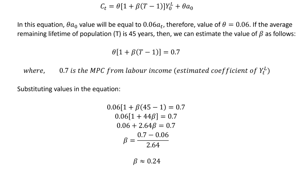
Positive coefficient beta  suggests that with an increase in current labour income, the average expected labour income increases. As current labour income increases by $1, the average expected labour income increases by $0.25.

MPC and APC

This estimated consumption function has a slope of 0.7 or MPC, corresponding to the coefficient of Y t L . The intercept of the consumption function is equal to 0.06a t  because assets remain the same in the short run. As seen in the figure, APC is falling with a rise in labour income and MPC<APC in the short run consumption function.

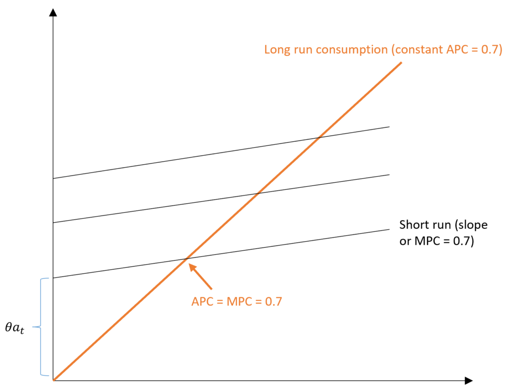
In the long run, however, assets will not be constant. With an increase in assets, the short-run consumption functions will keep shifting upwards as the economy grows. Therefore, long-run consumption will be along the trend where APC is constant and APC=MPC along this long-run consumption.

The APC will be constant if the share of labour income in total income ( Y t L / Y t ) and the ratio of total assets to total income (at / Yt) remain constant in the long run as the economy grows along the trend. Ando and Modigliani observed that both these ratios remained fairly constant in the long run in the annual U.S. data. The labour share in income was around 75 per cent and the ratio of assets to income was around 3. Therefore, the estimated APC is:

criticism of Life-cycle Hypothesis

• The life cycle hypothesis assumes that everyone is a rational consumer aiming to maximize utility based on expected income. However, this may not be necessarily true because not everyone’s consumption decisions are based on future income. Some individuals may not even consider future outcomes while spending in the current period. Or they may be impulsive and lacking in self-control. And, they do not focus on having a smooth consumption over a long period.
• The life-cycle hypothesis assumes that every increase in current income leads to an increase in average future expected income. This may not be true in every case because every income change will not necessarily affect expected future income. For instance, a temporary tax that changes current income, but, consumers are aware that it is temporary and they will not change their expected future income.

Nevertheless, life-cycle theory explains consumer behaviour across cross sections, short run as well as long run. Additionally, it takes into account the role of wealth or assets in determining consumption and can be empirically tested.

You Might Also Like

Relative income hypothesis, absolute income hypothesis, difference between microeconomics and macroeconomics, leave a reply cancel reply.

To provide the best experiences, we and our partners use technologies like cookies to store and/or access device information. Consenting to these technologies will allow us and our partners to process personal data such as browsing behavior or unique IDs on this site and show (non-) personalized ads. Not consenting or withdrawing consent, may adversely affect certain features and functions.

Click below to consent to the above or make granular choices. Your choices will be applied to this site only. You can change your settings at any time, including withdrawing your consent, by using the toggles on the Cookie Policy, or by clicking on the manage consent button at the bottom of the screen.

Open Access is an initiative that aims to make scientific research freely available to all. To date our community has made over 100 million downloads. It’s based on principles of collaboration, unobstructed discovery, and, most importantly, scientific progression. As PhD students, we found it difficult to access the research we needed, so we decided to create a new Open Access publisher that levels the playing field for scientists across the world. How? By making research easy to access, and puts the academic needs of the researchers before the business interests of publishers.

We are a community of more than 103,000 authors and editors from 3,291 institutions spanning 160 countries, including Nobel Prize winners and some of the world’s most-cited researchers. Publishing on IntechOpen allows authors to earn citations and find new collaborators, meaning more people see your work not only from your own field of study, but from other related fields too.

Brief introduction to this section that descibes Open Access especially from an IntechOpen perspective

Want to get in touch? Contact our London head office or media team here

Our team is growing all the time, so we’re always on the lookout for smart people who want to help us reshape the world of scientific publishing.

Home > Books > Macroeconomic Analysis for Economic Growth

The Life Cycle Hypothesis and Uncertainty: Analyzing Aging Savings Relationship in Tunisia

Submitted: 13 August 2021 Reviewed: 15 September 2021 Published: 03 January 2022

DOI: 10.5772/intechopen.100459

Cite this chapter

There are two ways to cite this chapter:

From the Edited Volume

Macroeconomic Analysis for Economic Growth

Edited by Musa Jega Ibrahim

To purchase hard copies of this book, please contact the representative in India: CBS Publishers & Distributors Pvt. Ltd. www.cbspd.com | [email protected]

Chapter metrics overview

503 Chapter Downloads

Impact of this chapter

Total Chapter Downloads on intechopen.com

Total Chapter Views on intechopen.com

This research empirically checks the effect of uncertainty on aging-saving link that is indirectly captured by an auxiliary variable: the unemployment. It looks at the nexus population aging and savings by bringing out the unemployment context importance in determination saving behavior notably in a setting of unavailability of unemployment allowance. To better estimate population aging, it considers the old-age dependency ratio besides the total dependency one, which is the usually indicator used. Applying the Structural VAR model, the variance decomposition technique and the response impulse function, on Tunisia during 1970–2019, it puts on show that elderly do not dissave in a context of enduring unemployment and unavailability of unemployment allowance. Unemployment is an important factor able to shaping the saving behavior and to distort the life cycle hypothesis’s prediction. Consequently, the life cycle hypothesis cannot be validated under uncertainty. Hence, aging does not to alter savings systematically. The nature of aging-saving relationship is upon to social and economic context.

• Unemployment
• life cycle hypothesis

Author Information

Olfa frini *.

• ISCAE, University of Manouba, Tunisia
• ECSTRA Lab, Carthage University, Tunisia

*Address all correspondence to: [email protected]

1. Introduction

There is a great concern about the increase of elderly proportion follow-up the aging population process over the world. It is likely to create important macroeconomic issues and involve new policies challenges as it will put downward pressure on saving according to the life cycle hypothesis (LCH) prediction formulated by Modigliani and Brumberg [ 1 ]. Indeed, the saving decline is well recognized to be associated with lower rates of capital accumulation and growth in the economy. Saving is crucial for investment and the maintenance of strong and sustainable economic growth. In addition, saving is one of the essential aspects of building wealth and having a secure financial future. It gives a way out from uncertainties of life and enjoy a quality of life.

Hence, it is of great interest to look at the demographic changes impact on saving in order to seek how to prevent saving from such an eventual decline. The empirical studies in the topic, generally, have relied on the life cycle model; as it better explains the varying rates of savings in societies with relatively younger or older populations. However, the LCH’s prediction was not often empirically validated to argue that saving will be automatically depressed consequence of the population aging process. There is evidence that the social and economic conditions limit the scope of the LCH.

This study reviews the LCH to emphasize the most significant factors that may distort its prediction. It focuses on the uncertainty to explain the aging-saving relationship. It tries to check empirically whether uncertainty consideration may distort the LCH. Thereby the aging population do not put a down pressure on saving systematically.

However, given the difficulty to directly and objectively estimate uncertainty extent on saving behavior, we indirectly capture by an auxiliary variable the unemployment. We seek to highlight the influence of the precautionary motive related to the risk of unemployment. Thus, we try to give information about the transmission mechanism between aging population and saving considering the unemployment savings pattern as a determinant of saving behavior in a setting of unavailability of unemployment allowance. So, we draw attention that unemployment is an important factor up to distort the life cycle model’s prediction.

Unlike previous studies, we build our estimates not only on the total dependency ratio (the proportion of population aged less than 15 years and aged 60 years or more versus the proportion aged 15–59) as an aging indicator, but also on the old-age dependency ratio (the proportion of population aged 60 years or more versus the proportion aged 15–59). This will allow us to make comparison and to deduce the effect of the child dependency ratio (the proportion of population aged less than 15 years versus the proportion aged 15–59). Besides, we focus on national saving to avoid narrowing the population aging impacts since the corporate and the government saving are sensitive to population aging as the household saving.

In addition, given the lack of researches on this issue on developing countries (which economic and social environment greatly differ from the developed countries) we devote our study to Tunisian case. Tunisia is an interesting case of study because it is a well advanced in the aging process. As well, it suffers from an enduring and high unemployment rate and an inefficient pension system (as detailed in Section 3). Furthermore, it is characterized by a strong altruistic familial intergenerational relationship [ 2 , 3 , 4 ].

To check out the relationship between aging, unemployment, national saving and economic growth we apply a time series modeling approach over the period 1970–2019. We carry out a Structural VAR model, as defined by Sims [ 5 ]. We analyze the impulse response functions (IRFs) of different shocks for all variable’s fluctuations. We also apply the bootstrap methods to construct the confidence intervals of the IRFs. Additionally, we complete our dynamic analysis by the variance decomposition.

This study represents the first attempt to model the Tunisian aggregate national saving by considering both the impact of demographic changes and of unemployment.

In what follows, we give, in Section 2, an overview of the life cycle hypothesis and its bounds. In Section 3 we give some sight of the demographic change and the saving evolution occurred in Tunisia. In Section 4, we specify the econometric model and in Section 5 we discuss the results found. Finally, we end, in Section 6, with the main findings and policy recommendations.

2. Life cycle pattern overview

In this section we state the life cycle’s savings to emphasize the social and economic conditions that may constrain its validation.

2.1 Life cycle hypothesis

The life cycle theory pinpoints the intertemporal allocation of time, effort and money. In its simple form, the standard life cycle hypothesis’s (LCH) formulated by Modigliani and Brumberg [ 6 ], suggests that individuals save during working life for their consumption needs when they retire, dissave after retirement, and die without wealth. Hence, individuals will smooth consumption over their lifetime regard to the expected lifetime resources. They accumulate wealth during the pre-retirement period by consuming less than their disposable income. So, during retirement, they de-cumulates wealth to finance its consumption. That is, the saving rate should follow a hump-shaped over the life cycle as shown by the Figure 1 (in the Appendix).

Therefore, one very important implication of the LCH is that the demographic profile of a population should be an important factor influencing the aggregate saving rate. Given that population aging is defined as a shift in the population age distribution towards old age, so a change of the balance between youth and elderly proportion (defined in the following as a person aged over 60 years-old) causes society to age and subsequently to affect the saving pattern. 1 Such a change may change the savers proportion in the economy and diminish the aggregate saving rate according to the LCH.

If there is a large proportion of the population working, then, the saving rate should be high. However, if there is a large population proportion over retirement age or very young, the saving rate would be low. This suggests that aggregate saving rate should be negatively correlated with total dependency ratio.

Even though the theoretical conclusion of the life cycle model is clear, the empirical evidence is not often proved and stays controversial until today as it was decades ago. There is evidence that elderly may not dissave, at least not to the extend hypothesis suggested by the pure life cycle model which abstracts a number of factors that would complicate its prediction.

2.2 The life cycle hypothesis bounds

The Life cycle theoretical conclusion is understandable given its simplifying assumptions such as no uncertainty, a finite decision horizon, no inheritance and perfect financial market with no credit constraint [ 7 ]. According to the LCH, individual takes decisions basically depending to events and fact that are known with certainty in each period of life (such future income, death date, and interest rate). Nevertheless, these assumptions are considered too restrictive. Indeed, events are uncertain [ 8 , 9 ] and financial market is imperfect with credit constraint. Uncertainty affects consumption and savings behavior as consumers are generally cautious. Moreover, according to the Kotlikoff [ 10 ] dynastic model of savings, individuals do not act in a finite horizon, but in an infinite one. In addition, they have a dynastic behavior characterized by a strong preference to let, at their death, a very limited capital de-cumulation [ 11 , 12 , 13 ]. Thus, parents, having an altruistic motive, seek to not decumulate wealth to leave inheritance to their children. Consequently, the population aging may not automatically depress national saving. Kotlikoff and Summers [ 14 ] conclude that the “life cycle saving” cannot account for more than 20 percent of U.S. capital formation, and the intergenerational transfers play a dominant role in wealth accumulation, accounting for 80 percent or more of observed wealth.

Additionally, it is worth noting that the conflicting evidence on the life cycle saving may also be due to the econometric approaches used and the aging indicator chosen. Indeed, the micro econometric analysis invalidates life cycle model’s prediction to support the Kotilkoff hypothesis but their results are difficult to aggregate because of severe problem of heterogeneous behavior at the household level. Conversely, studies based on macro data for a country generally support the prediction. However, most of them refer to developed societies while in developing societies people face different economic challenges and social conditions, which may lead to different evidences. In that way, these studies could not be very useful for understanding saving behavior in developing countries. The difference through countries is in the design of pension systems and health care, taxes and transfers as well as labour market conditions, which are unavoidably depend to the population age distribution. As well, they may alter individual economic behavior and so could be the origin of the inconsistency LCH’s evidences.

Also, the choice of the population aging indicator to estimate is crucial. The total dependency ratio which is generally used does not accurately reflect the aged population since it composed of both the old and the child dependency ratio. It is more fitting to use the old-age dependency ratio to explicitly consider the effect of aged population on savings rate [ 15 ]. With more cautious in the aging indicator use, the life cycle model’s prediction is likely to be endorsed also in macroeconomic approach.

2.3 The life cycle hypothesis and uncertainty

The LCH analysis has been gradually enriched, to focus on three reasons for accumulation: the foresight for retirement, the intergenerational altruism and inheritance and the wariness of the saver face to risk (of income, health and lifetime span). In this work, we focus more on the third reason of accumulation by looking at how uncertainty, about future income affects the behavior of the individual’ saving. Uncertainty consideration has made it possible to highlight precautionary behavior as the future work income is random; consumption (otherwise savings) depends not only on expectation, but also on the variance of the expected income. A risk-averse or aware consumer will save more. In fact, savings play an insurance role against the hazards affecting the household, especially the hazards related to income (unemployment, loss of wages, etc.) [ 16 ]. Thus, uncertainty about future income affects the behavior of the individual ‘saving by increasing the demand for precautionary assets, and hence savings amount.

As well, there is precautionary behavior as to face health care expenditure at advanced aged when the risk of health problems is potentially great; notably in the context of inefficient health care system [ 17 ]. As a result, households are saving not only to offset lower future income, but also to insure against all sorts of risks.

However, empirically it is not easy to estimate uncertainty extent on saving behavior. It is difficult to quantify this relationship given the difficulty to directly and objectively estimate uncertainty. Empirically there are no quantitative measurements of uncertainty that could be used directly. In the case studies, income uncertainty is usually measured indirectly by auxiliary variables such as inflation rate, unemployment rate or a derivative of these variables. In this case of study, we focus on unemployment as an income uncertainty indicator to better understand the aging impact on saving and to find an answer to the crucial question: do population aging depress savings?

Unemployment inevitably alters the savings behavior by its two aspects: (1) a high rate and (2) an increase in the average age of unemployed [ 18 ].

(1) The high and persistent unemployment rate weights on household confidence, prompting them to increase their precautionary savings. Such behavior is accentuated in a setting of unavailability of unemployment allowance (like in Tunisia) [ 19 ]. Thus, for precautionary reasons and to finance unexpected income losses, unemployment is viewed as an income uncertainty given the probability to become unemployed alters the savings behavior. Faure et al. [ 20 ] shown that unemployment and the deterioration of household confidence accounted for almost 20% of the aggregate consumption decline.

(2) The increase of the unemployed average age implies that the working population becomes occupied at advanced age. Consequently, they would save a less amount of wealth and they would form a low retirement pension. To offset at this lack of savings they do not immediately dissave at the beginning of the retirement. They would even compensate their low pension by working further after retirement, mainly at the beginning of the period (as long as they stay in better health) to face the future’ uncertainties. Also, given the granting difficulties for credit liquidity at the retirement period, this insufficient pension nudges them to continue to save to keep up a certain level of consumption. It increases, in addition, the need for retirement savings from private sources.

Furthermore, the high and enduring unemployment increases inter-vivos transfers, which represents a form of precautionary saving [ 21 ]. With a dynastic behavior (which is ignored by the LCH) the old generation (parents) saves more throughout the life cycle to help the young generation (their offspring) to facing uncertainty and hard-economic conditions related for instance to unemployment’s conditions. Thus, if intergenerational transfers (by purely altruistic incentive or following a kind of implicit contract between parents and children) are an important motive for savings; elderly rarely decumulate their wealth.

Henceforth, given uncertainty about the future income and lifespan, liquidity constraints, and the wish to leave bequests (a dynastic savings) population aging would not drive the decrease of savings. Therefore, aging economic impact on the household saving and so on the cumulative and on national saving, may not be large [ 22 ].

Hence, for our empirical evaluation of the life cycle hypothesis, we analyze the aging-savings relationship in a developing country, in particular, Tunisia. It greatly differs, economically and socially, from the developed countries, by its altruistic familial intergenerational relationship, the enduring and high unemployment rate and the inefficient pension system; as detailed in the section below.

3. The Tunisian demographic and economic setting

3.1 demographic shifts and age structure evolution.

Tunisia after has shortly ended its demographic transition regime, it has well undertaken the population aging process. During the period 1960–2019, the mortality rate fell from 35 to 40 per thousand to a low rate 5.9. Likewise, fertility which was nearby 8 children per woman fell to 2.17. Thus, the life expectancy has attained an average close to that of developed countries 75.4 years (78.1 years for woman and 74.5 years for man) in 2017.

Accordingly, the population age distribution has shifted towards aging. This fertility decline has narrowed the bottom of the age pyramid by the decline of the younger generation size, while the mortality decline has enlarged the top of the pyramid through the life expectancy gain. Thus, the age range proportion less than 15 years-old becomes less important (passing from 46.5 percent to 24.7) and it is likely to continue its decline. In the contrary, a remarkable increase is recorded for the proportion of person aged over 60 years-old (from 5.5 percent to 12.6) and is expected to increase by 10 points over the future three decades. Therefore, during 1966–2019, the child dependency ratio has sharply declined (from 96.27 percent to 39.36) while the old-age dependency ratio has increased (from 11.60 percent to 20.08). Consequently, the total dependency ratio has decreased (from 107.86 percent to 59.44).

3.2 Economic setting

Tunisian economy recorded a high and enduring unemployment. Over the period 1966–2000, it has increased by 6.1 points to pass from 12.5 percent to 18.6, and then fell slightly to stabilize during the last two decades (2000–2019) around 15.3 percent. Additionally, aging has hit the age composition of the unemployed. Indeed, the modal age range of the unemployed population has moved from less than 25 years-old (by about 29 percent) to 25–29 years-old (by about 34.2 percent) during 2005–2011. It is worth noting here that Tunisian authorities do not distribute any unemployment allowance. 2

For the national saving, it has evolved with some fluctuations. During the period 1970–2010, the national saving rate (of gross national disposable income) was relatively stable around an average of 22.8 percent then progressively fell to achieve 9.3 in 2019, mainly due to a steady loss of purchasing power. 3

According to the Islamic Development Bank, the behavior of Tunisian investors appears to be driven by factors related to consumer demand and/or the income effect [ 23 ]. The financial changes in interest rates have more effect on the savings structure than on its volume. Indeed, the financial liberalization policy adopted (since the structural adjustment plan in 1986) has not succeeded to stimulate private savings through the increasing of the real interest rates [ 24 ]. In Tunisia, saving behavior seems to comply more to the Keynesian approach.

However, an interest for the long-term financial savings is recorded. During 2010–2017, the listed companies increase from 56 to 81 with a broad sectors diversification. Likewise, the life insurance, as a long-term saving vehicle, has undergone an important increase; the average annual growth rate was 18 percent in 2017. Its share in the insurance market has climbed from 12.05 percent in 2009 to 20.2 in 2017; however, it remains far from the international standards (about 56.2 percent).

This interest for the long-term savings is explained by the failure of the pension system the pay-as-you-go system and the bankruptcy of the provident fund as well as the authority’s future intention to withhold a proportion of the retirement pension. 4 Thus, the insured people are driven to form a complementary retirement pension under others retirement savings forms through voluntarily paying into saving schemes in private financial institutions. This savings form is encouraged by the financial authority through the establishment of tax benefits.

Concerning the non-financial savings, it is allocated to buy housing, jewelry or land by household and productive assets by individual corporate. Household saving is particularly oriented to housing savings which has experienced a growth rate of about 5.5 percent during 2000–2017.

4. Econometric model and data specification

To look at the relationship between population aging and savings in an unemployment context in Tunisia over the period 1970–2019, we apply a structural VAR model, as defined by Sims [ 25 ]. This enables us to approach a multivariate causal setting allowing the coexistence of both short and long-term forces derived from the aging influences on saving decisions. Finally, we deepen our dynamic analysis by application the techniques of impulse response functions (IRFs) of different shocks for all variable’s fluctuations and of the variance decomposition (VDC).

4.1 Data specification

To undertake the aggregate saving model estimating, we use as an independent variable the national savings rate unlike previous studies, which generally referred to the household savings rate. National saving is important as it is a source of investment and one of the major determinants of macroeconomic growth. Also, as it is closely related to the demand for financial and real assets and it may affect asset price formation. In addition, we seek to avoid narrowing the aging impact as its takes into account companies and public sector saving (related to social sector, health, education and pensions). On another side, the household savings refers to survey measure which undervalues personal income as it provides information related to expenditure than to income sources. Likewise, it does not capture the same share of total saving for persons at different ages, so the estimate of relationship between savings and age may be fallacious.

As a definition, between the two known alternative measures of savings (S) we adopt that of national account (as income minus consumption expenditure) given data availability. 5 Explicitly, we use the savings rate with respect to the gross national income disposable income 6 .

For independent variables, we refer to the main population aging indicators. We consider the mortality rate (MR) and fertility rate (FR) to capture demographic changes and its impact on the age structure composition, and likewise on the dependency ratio. We consider the old-age dependency ratio (EDR) to accurately look at the effect of aging besides the broadly used the total dependency ratio (TDR). Then, we could deduce if the aging impact is due to the fertility decline or to the longevity increase.

Concerning economic variables, we include three macroeconomic variables. (1) Basing to the neoclassical approach we introduce the interest rate (MMR) in particular the money market rate as a driver of the real interest rate (credit and debit). (2) As a one quantitative measure of aggregate income uncertainty we consider the aggregate unemployment rate (U). (3) In order to check the economic effect of saving, we examine the economic growth (G) measured by the GDP per capita at constant domestic prices. It is computed by dividing GDP per capita at current domestic prices by the consumption price index (base 1990). Hence, the inflation rate is indirectly considered.

The main statistical characteristics of these variables used are summarized in Table 1 (in the Appendix). Data are drawn from the Central Bank of Tunisia (CBT), the National Institution of Statistics (NIS) and Tunisian Institute of competitively and quantitative study (ITCQS).

4.2 Econometric models

Our analysis is based on the identification and estimation of structural vector autoregressive (SVAR). The SVAR model is used in macroeconomic analysis in order to check the effect of exogenous shocks (of the demographic change, for instance) on macroeconomic variables.

Our basic model VAR is the following:

where Y t is a column vector of stationary variables considered in the estimate.

The selection and order of independent variables are essential in the SVAR estimate. Thus, the independent demographic variables are introduced with caution following the demographic transition theory. As mortality decline brings that of fertility, so we first introduce the mortality rate (MR) followed by the fertility rate (FR). ​ Then, we integrate the dependency ratio as an indicator of the population aging and the age structure change following the demographic transition.

After what, we consider the economic variable exogenous effect on saving. So, we insert the interest rate (MMR) as a saving determinant and the aggregate unemployment rate (U) as a measure of aggregate income uncertainty. Lastly, we introduce the national savings rate (S) followed by the economic growth (G) to check the aging impact on economic growth through the savings evolution.

As we use two dependency ratios, we estimate two distinct vectors autoregression. A vector includes the total dependency ratio which reflects the effect of both the mortality and fertility evolution as a result of the demographic policy as follows (MR t , FR t , TDR t , U t , MMR t , S t , G t ).

The second vector includes the old-age dependency ratio and takes the mortality choc as the main cause of the elderly proportion evolution as follows (MR t , EDR t , U t , MMR t , S t , G t ).

Otherwise, Γ(L) = Γ 1 L 1  + Γ 2 L 2  + … + Γp. L p is a lag operator in the form of polynomial matrix and ν t is a vector of idiosyncratic errors, where ν t = (μ 1 t ,…,μ 5 t ) ’ . These errors are not auto correlated and are homoscedastic. Then, the representation (1) can be written in the form of a moving average of infinite order VMA (∞) (representation theorem of Wald):

where C(L) = [I - Γ(L)] −1 .

The structural form (SF) of the model (1) can be written as follows:

where A(L) = C(L) H is the coefficient matrix (a ij ) of (7 × 7 or 6 × 6 for the two vectors respectively) size, and more precisely it represents the impulse response functions of the elements of Y t following the various shocks. Moreover, H is the transition matrix and ε is the vector of structural shocks where E (ε t ε t ’) = I N .

However, the identification of these shocks requires the Cholesky decomposition in the order to identify the structure of the shocks. As a result, the decomposition of the variance covariance matrix of the reduced form residuals is written in a lower triangular matrix A(L). The number of constraints imposed on A(L) is equal to 21 i.e. n × (n-1) / 2 with n = 7 variables and where some of the structural shocks do not have contemporaneous impact on other variables.

Additionally, the Cholesky decomposition assumes that series listed earlier in the VAR order impact the others variables contemporaneously. But series listed later in the VAR order impact those listed earlier only with lag. Therefore, the variables listed early in the VAR order are considered more exogenous. As mentioned above, the order of endogenous variables is central to the identification of structural shocks, i.e. it determines the structure of the shocks. More precisely, the first variable has impacts on all the variables that are below it, but it does not receive any impacts from these variables. This rule applies to all subsequent variables. For instance, the triangular matrix A(L), for the case of n = 7 variables, is as follows.

Henceforth, we have to estimate four matrixes: a matrix (Alt1) for the total dependency ratio and one for the old-age dependency ratio (Alt2). Two others matrixes are also estimates as a robustness test by omitting the unemployment rate, respectively the matrixes (Alt3) and (Alt4).

To undertake the SVAR estimate model, we first study the stationarity of all variables using the Phillips-Perron test [ 26 ]. As reported in Table 2 (in the Appendix) all the considered variables are I(0) suggesting that a long-run (cointegration) relationship could exist between the considered variables.

Then we determine the order p of the VAR process to remember. To do this, we consider various processes for VAR lag orders p ranging from 1 to 4. For each model, we calculate the Akaike information criteria (AIC) and Schwarz (SC), and the log-likelihood (LV) to hold the p lag (=4) that minimizes these criteria as indicated in Table 3 (in the Appendix).

Accordingly, four alternatives are estimated, respectively with the identification of cointegration relationships by using the cointegration test of Johansen [ 27 ] as well as the structural factorization (with 500 iterations).

Finally, to examine the dynamic of the model, we refer to the impulse response function (IRF). It helps us to judge and to appreciate the channel(s) of population age structure change transmission. It allows to see if there is really a robust, stable and predictable relationship between aging and savings. In this respect, we will identify the different responses of all the variables in the model to various shocks. It should be noted that we focused on the effects of the shock on 10 periods and that errors are generated by Monte Carlo with 100 repetitions. Such analysis is strengthened with the variance decomposition analysis (VDC), which however, indicates the proportion of the variable changes due to own shocks versus shocks on the other variables. Namely, the variance of the forecast error of the change in savings rate is partitioned among the contributions of the innovations in each variable of the system.

5. Results interpretation

Interestingly, results put forward that the LCH prediction is not automatically confirmed, but it is up to the economic uncertainty extent. Indeed, the LCH is not validated in the unemployment setting, which is considered in our study as an indirect measure of income uncertainty.

5.1 The SVAR results interpretation

The SVAR’s estimate results (reported in Table 4 in the Appendix) points out that uncertainty encourages saving. Indeed, for the two aging indicators used (TDR and EDR) the LCH prediction is not validated once unemployment is introduced unlike Ahmedova’s [ 28 ] findings. As we note from matrixes Alt1 and Alt2, the two indicators present a significant positive effect on savings rate in the context of enduring unemployment without allowance, like in Frini’ work [ 29 ]. However, this effect is found more significant for old-age dependency ratio, unlike in Wong and Tang [ 30 ] and Loumrhari’s [ 31 ] findings.

In contrast, the LCH prediction is validated by the estimate omitting the unemployment rate, however, for only the total dependency ratio. Indeed, a significant negative effect is found in the matrix Alt3.

Such results confirm that the demographic changes impact on saving depends on the perception of the economic context and the confidence towards future. Furthermore, the LCH’s validation appears to be, as well, empirically related to the aging indicator used in the estimate. This confirms our proposal that the old-age dependency ratio indicator seems more efficient to explicitly check the effect of aging.

The unemployment which hints uncertainty about future income pushes the savers to keep up savings. It reduces confidence and intensifies incentives for precautionary saving so that, it prevents savings from decline. Indeed, the unemployment rate displays a significant and positive coefficient. The weight of the future uncertainty boosts the employed population to form a precautionary savings. This precautionary saving is important to offset the small amount of wealth accumulated after an enduring unemployment without any allocation benefit. When enduring a long unemployment period and facing great difficulties for credit liquidity at old age, elderly try to continue to save to keep up a certain level of consumption. Such behavior is very pronounced in Tunisia since retired do not benefit from a sufficient pension in a distressed pay-as-you-go system. The insufficiency of pension and medical care benefits entails the elderly saving’s behavior adjustment by continuing to work and to save at the beginning of the retirement period (as long as they remain in better health). As pointed out by Frini [ 32 , 33 ] the new retirees or the youngest elderly (which share, generally, weighs more than that of the old retirees or the old elderly) maintain their savings mainly for precautionary motives in high uncertainty economic environment.

This Tunisian elderly saving behavior may in part be strengthened by the intentional transfers motivation of the old generation towards the young one. Indeed, Tunisian families, as stressed by Mahfoud [ 34 ] and Frini [ 35 , 36 ], are strongly linked and directed by an intergenerational altruistic motive. So, the old generation do not seek to cut savings so as to help the young generation to face uncertain environment and hard economic conditions.

As expected, mortality drop induces a fertility decline, putting on show the demographic transition theory. This fertility decline increases the savings rate. It seems that the youth share decrease outweighs the small increase in the elderly share since the aggregate savings rate increases. Household with fewer children are likely to incur less expenditure in respect to their income for looking after them and then would save more. In addition, a reduced family size leads to a competition between children as a mean of transferring income from present to future and as a financial asset. 7 Henceforth, by the fall of fertility rate, the demand of financial and capital market as a substitute of youth assurance service will increase and thus savings. Additionally, the decline of government expenditures for youth (given their share decline), seems to make up or even more the government expenditures increase for elderly (due to their share increase) to not lead savings decrease.

Considering uncertainty, mortality evolution positively influences savings rate when considering the economic and social facts, but negatively when they are neglected. The increase of mortality risk and health problem intensifies precautionary behavior to face health care expenditure at old age.

The uncertainty related to interest rate affects positively the savings rate. An increase in interest rate will make saving more attractive. Finally, like in AbuAl-Foul’s [ 37 ] work results show that no long-run relationship exists between saving and GDP growth. This in part due to that saving is, generally, done in real estate, which is known as a small creator of wealth with a small ripple effect.

5.2 The IRF’s and VDC’s results interpretation

Likewise, the IRF’s and VDC’s results underline that population aging on savings evolution changes respect to the economic uncertainty context. Savings positively respond to age structure changes once unemployment is taken into account. The different graphs of impulse responses ( Figure 2 in the Appendix) show that savings respond quickly to demographic changes (mortality rate, fertility rate and dependency ratio jointly), but weakly to the shock of the money market rate. The response due to unemployment rate shock can be judged as significant with a return to equilibrium in the long-term. The saving response to economic growth innovations is, however, slow and limited. This analysis is corroborated out by the variance decomposition as displayed in Table 5 (in the Appendix). 8 In detail, a relatively constant proportion of the change in savings rate variance is recorded for both ratios. The total dependency ratio shock is by about 3.75 percent for Alt1 and by 4.26 percent for Alt3 after three years. The old-age dependency ratio shocks are, however, of a less proportion by 1.42 percent for Alt2 and 0.16 percent for Alt4 over ten years. The noteworthy result is that savings evolution follow-up a shock of the total dependency ratio is more significant (by three times more) than of the elderly one. This fact is also proved by the dynamic response path. Fewer children lower the dependent population and consumption without contribution to income. The decrease of the youth dependent proportion out weights the increase of the elderly dependent in the proportion, which limits saving rate depression. This brings up the role of relative weight of the youth share to the elderly share on savings evolution. Further, the increase of elderly proportion appears not to cut savings rate. Thus, savings rises when fertility declines and longevity increases, but less intensively. In the contrary, to the LCH prediction, the old-age dependency ratio shock instantaneously and positively affects saving rate, however, more weakly than the total dependency ratio.

Remarkably, once we ignore the labour market unbalance (or uncertainty) of the estimates the relationship between aging and savings becomes consistent with the LCH prediction. The total dependency ratio shocks present a negative short-term impact on saving to disappear at long-run (after eight years). However, no impact is found for the old-age dependency ratio. This discrepancy in estimated magnitude through the two dependency ratios used refers back to our assumption that aging impact may be sensitive to the measurement used to describe it.

Moreover, demographic indicators shocks trace the variance of savings innovations. Mortality rate explains saving variance by almost the same small proportion (by about 2.30 percent) for all alternatives in the variance decomposition, but relatively less without the unemployment rate. In the impulse function graph, a negligible positive impact is found of mortality shock. Hence, with the rise of longevity and elderly proportion savings may not decline. Fertility decline significantly contributes in the savings change variance (by about 5.16 percent in Alt1) and even much more when forsaking the unemployment rate (by about 17.79 percent in Alt3). The corresponding impulse function displays a negative influence over six years to reverse positively after.

However, saving is less sensitive to interest rate shock. Money market rate contribution is more pronounced for the total dependency ratio than the elderly one. The same evidence is observed through the impulse function graph shown a very small positive influence which disappears in the long-term. This small impact of the real interest rate on saving may hide the offsetting of its two effects (of income and substitution). In other hand, it may be related to the Tunisian household’s behavior which seems to comply more with the Keynesian approach.

Finally, in the long-term, savings shocks seem to produce an effect on economic growth, but weakly when the imbalance labour market is considered (as reported in Table 6 in the Appendix). As mapped out by the response functions this dynamic is non-instantaneous. In contrast, a very small ‘feed-back’ seems to be produced of economic growth over three years on saving.

6. Conclusion

This study puts on show that the life cycle prediction of a downward pressure on saving by aging population could not be proved under uncertainty. Population aging is, on contrast, found to exert a long-term upward pressure on saving in an unemployment context. The economic environment’s uncertainty (such income uncertainty) quantified, in our case of study, by the unemployment phenomenon, looks to be an essential factor of the change in the life cycle pattern of savings. It is able to shaping the saving behavior and to distort the LCH. The impact of the demographic change seems strongly related to the economic confidence factors. Accordingly, the social and economic conditions limit the scope of the LCH. Thus, population aging will not necessarily spell disaster on national saving. Consequently, studies’ findings on developed countries could not be representative of saving behavioral in developing countries; where pension and medical insurance schemes are less developed and the persistent unemployment is without unemployment allowance benefit. Furthermore, it seems that the empirical findings checking the LCH depend on the aging indicator used. In fact, the use of the total dependency ratio could not validate the LCH, but it is validated by the old-age dependency ratio use. So, with more caution on the population aging measure, the evidence that elderly do not dissave may be found and the life cycle prediction may not be endorsed. Henceforth, the life cycle hypothesis may not be validated in macroeconomic approach as in the micro-econometric approach.

Finally, as policy implications, several measures are needed to sustain saving rate or to prevent it from an eventual decline. In addition to the strategy applied lately to postponing the retirement age to 62 years-old, Tunisian Policy-makers have to accelerate the move from the pay-as-you-ago public pension system towards the funded pension system to cut costs of increasing old-age benefits. As well, to mobilize more savings, they should shift the liquid savings towards long-term products. Accordingly, it is important to reconsider the long-term savings strategy to meet the household’s needs as well as the huge potential investment’s needs. Therefore, major economic and financial reforms should be undertaken to restructure public corporates and the partial openness of their capital, to strengthen the pension plans, to develop the insurance sector and promote life insurance, and to improve the framework of the stock market and the bond market and diversify product of savings.

Consumption,consumer income, wealth and saving over the life cycle.

Descriptive statistics variables.

Unit root test of ADF.

Note: The null hypothesis for the ADF test is that the series are non-stationary i.e. there is presence of unit root. The values ​​in the table indicate the p-values ​​of this test. Using the Phillips-Perron test, the results were the same.

* and **denotes that the null hypothesis of unit root is rejected at the 5% level and 10% level respectively.

Choice of the lag number of VAR (p) process.

Note: LV denotes the log-likelihood; the asterisk indicates P order to retain according to the criterion used.

SVAR estimates results for the four alternatives.

Variance decomposition of saving rates (Cholesky ordering).

Notes: Cholesky ordering follow that of the four alternatives. The second column (S.E) shows the forecast error of the variable at the given forecast horizon. The source of this forecast error is the variation in the current and future values of the innovations to each endogenous variable in the VAR. The other columns give the percentage of the forecast variance due to each innovation.

Variance decomposition of economic growth to saving rates.

Estimated impulse response functions. Response to Cholesky one S.D. innovations.

Classifications

JEL Classifications: J1, E2, C3

• 1. Modigliani, F. & Brumberg, R. (1954). Utility Analysis and the Consumption Function: An Interpretation of Cross-section Data’ Post Keynesian Economics , ed Kenneth K. Kurihara. New Brunswick: Rutgers University Press.
• 2. Frini, O. (1996). Le transfert intergénérationnel et accumulation du capital humain: cas de la Tunisie . A search dissertation.
• 3. Frini, O. (2014). The Familial Network Influence on Fertility Behaviour in Tunisia. Journal of Economic and Social Research, 16(1–2), 33-61
• 4. Mahfoud Draoui, D. (2006). Entraide familiale et nouvelles formes de solidarité’, 2 ème table ronde des cercles de la population et de la santé de la reproduction; “dynamiques familiales et solidarités intergenérationnelles” ONFP, Tunis 24 February 2006.
• 5. Sims, C (2002). Solving Linear Rational Expectations Models. Computational Economics 20, 1–20.
• 6. Modigliani, F. & Brumberg, R. (1954). Utility Analysis and the Consumption Function: An Interpretation of Cross-section Data’ Post Keynesian Economics , ed Kenneth K. Kurihara. New Brunswick: Rutgers University Press.
• 7. Attanasio, O. & Weber, G. (2010). Consumption and Saving: Models intertemporal Allocation and their implication for Public Policy. Journal of Economic Literature, 48(3), 693-751. http://www.nber.org/papers/w15756.pdf
• 8. Leland, H. (1968). Savings and Uncertainty: The Precautionary Demand for Savings. The Quarterly Journal of Economics 82, 465-473.
• 9. Nagatani, K. (1972). Life Cycle Savings: Theory and Fact, American Economic Review 62(1), 344-353.
• 10. Kotlikoff, L. (1988). Intergenerational Transfers and Savings, Journal of Economic Perspectives 2, 41-58. DOI: 10.1257/jep.2.2.41.
• 11. Ameriks J., A., Laufer, C., S. & Van Nieuwerburgh, S. (2011). The Joy of Giving or Assisted Living ? Using Strategic Surveys to Separate Public Care Aversion from Bequest Motives. The Journal of Finance, 66(2), 519-561. https://doi.org/10.1111/j.1540-6261.2010.01641.x
• 12. Lockwood, L. (2016). Incidental Bequests: Bequest Motives and the Choice to Self-Insure Late-Life Risks. NBER Working Paper No. 20745.
• 13. De Nardi, M., French, E., & French, J. (2016). Medicaid Insurance in Old Age. The American Economic Review, 106(11), 3480-3520. http://dx.doi.org/10.1257/aer.20140015 .
• 14. Kotlikoff, L. J. & Summers, L. H. (1981). The Role of Intergenerational Transfers in Aggregate Capital Accumulation, Journal of Political Economy 89 (4), 706-732.
• 15. Ahmedova, D. (2011). The impact of population Ageing on Private Savings Rate: Empirical Evidence from the OCDE Members Countries. Department of Economic, Central European University.
• 16. Antonin, C. (2018). Les liens entre taux d’épargne, revenu et incertitude. Une illustration sur données françaises . Documents de Travail de l’OFCE 2018-19. Observatoire Français des Conjonctures Economiques.
• 17. De Nardi, M., French, E., & Jones, J. (2010). Why Do the Elderly Save? The Role of Medical Expenses’, Journal of Political Economy, 118(1), 39-75. DOI: 10.1086/651674.
• 18. Kessler, D., Perelman, S., & Pestieau, P. (1993). Savings behavior in 17 OECD countries. Review of Income and Wealth Series, 39, (1)
• 19. Engen, E. M., & Gruber, J. (2001). Unemployment insurance and precautionary saving. Journal of Monetary Economics, 47 (3), 545-579.
• 20. Faure, M-E., Soual, H., & Clovis, K. (2012). La consommation des ménages dans la crise. Note de Conjoncture : 23–37.
• 21. Kotlikoff, L.J., & Spivak, A. (1981). The Family as an Incomplete Annuities Market. Journal of Political Economy, 89(2), 372-391.
• 22. Yamauchi, N. (1996). The effects of Aging on National Saving and Asset Accumulation. National Bureau of Economic Research (NBER) , Inc , 131-151.
• 23. BID, Thomson Reuters, IIRF and CIBAFI (2013) Tunisie prudemment optimiste Rapport pays sur la finance islamique, Retrieved from : http://www.irti.org/irj/go/km/docs/documents/IDBDevelopments/Internet/English/IRTI/CM/downloads/Reports/Tunisia_Islamic_Finance_Country_Report_Cautiously_Optimistic_Fr.pdf/
• 24. Tunisian Professional Association of Banks and Financial Institutions (2005) ‘L’épargne’, Retrieved from: http://www.apbt.org.tn/upload/telechargement/
• 25. Sims, C (2002). Solving Linear Rational Expectations Models. Computational Economics 20, 1–20.
• 26. Phillips, P. C. B., & Perron, P. (1988), Testing for a Unit Root in Time Series Regression, Biometrika, 75, 335-346.
• 27. Johansen, S (1988) Statistical analysis of cointegration vectors, Journal of Economic Dynamics and Control 12, 231-254.
• 28. Ahmedova, D. (2011). The impact of population Ageing on Private Savings Rate: Empirical Evidence from the OCDE Members Countries. Department of Economic, Central European University.
• 29. Frini, O. (2021). The relationship aging of the population and saving in an unemployment context: Empirical evidence using an autoregressive distributed lag bounds testing approach. Australian Economic Papers, 60(1), 98-121. DOI: 10.1111/1467-8454.12195.
• 30. Wong, B. & Tang, K.K. (2013). Do Ageing Economies Save Less? Evidence from OECD Data, International Journal of Social Economics, 40(6), 591-605.
• 31. Loumrhari, G. (2014). Ageing, Longevity and Savings: The Case of Morocco, International Journal of Economics and Financial Issues . 4, 344-352.
• 32. Frini, O. (2018). Do elderly really dissave? Empirical analysis using ARDL and NARDL bounds approach’4 èmes Journées Economiques et Financières Appliquées; Mahdia Tunisia 11 - 12 May 2018.
• 33. Frini, O. (2021). The relationship aging of the population and saving in an unemployment context: Empirical evidence using an autoregressive distributed lag bounds testing approach. Australian Economic Papers, 60(1), 98-121. DOI: 10.1111/1467-8454.12195.
• 34. Mahfoud Draoui, D. (2006). Entraide familiale et nouvelles formes de solidarité’, 2 ème table ronde des cercles de la population et de la santé de la reproduction; “dynamiques familiales et solidarités intergenérationnelles” ONFP, Tunis 24 February 2006.
• 35. Frini, O. (1996). Le transfert intergénérationnel et accumulation du capital humain: cas de la Tunisie . A search dissertation.
• 36. Frini, O. (2014). The Familial Network Influence on Fertility Behaviour in Tunisia. Journal of Economic and Social Research, 16(1–2), 33-61.
• 37. AbuAl-Foul, B. (2010). The Causal Relation between Savings and Economic Growth: Some Evidence from MENA Countries’, The 30 Th MEEA Meeting Atlanta .
• Population aging arises from two demographic phenomena the birth and the mortality decline. As for declining fertility, it reduces the number of children, which is generally considered a main explanation of growing aging. For mortality decline, it increases the longevity and the number of elderly.
• Source: NIS employment 1966, 2005, 2007, 2010, 2011.
• During 2011–2019 inflation rate has passed from 3.7 percent to 6.2.
• For instance, during 2010–2017, the overall financial situation of the three funds of the social security recorded a very serious drop going from 40MD in 2010 to −1326 MD.
• The second defines savings as the changes in net wealth. Net wealth accumulation includes capital gains and losses, adjusted for general inflation, and is more relevant for purposes of measuring changes individual’s economic well-being.
• Gross national income equal to the gross national income minus the current transfers (current taxes on income and wealth, social security contributions, social security benefits) paid to non-residents units plus the current transfers received from the rest of the world by the residents.
• Children is treated as pure capital goods and a kind of safety assets which returns are “elderly assurance”.
• The VDC indicates the proportion of the variable changes due to own shocks versus shocks on the other variables. The Cholesky decomposition method is used in orthogonalizing the innovations across equation. Percentage of forecast variances is explained by innovations.

© 2021 The Author(s). Licensee IntechOpen. This chapter is distributed under the terms of the Creative Commons Attribution 3.0 License , which permits unrestricted use, distribution, and reproduction in any medium, provided the original work is properly cited.

Continue reading from the same book

Published: 28 September 2022

By Ombeswa Ralarala and Masenkane Happiness Makwala

70 downloads

By Maria Letizia Bertotti

256 downloads

By Meng Sun

557 downloads

Top 4 Types of Hypothesis in Consumption (With Diagram)

The following points highlight the top four types of Hypothesis in Consumption. The types of Hypothesis are: 1. The Post-Keynesian Developments 2. The Relative Income Hypothesis 3. The Life-Cycle Hypothesis 4. The Permanent Income Hypothesis.

Hypothesis Type # 1. The Post-Keynesian Developments:

Data collected and examined in the post-Second World War period (1945-) confirmed the Keynesian consumption function.

Time series data collected over long periods showed that the relation between income and consumption was different from what cross-section data revealed.

In the short run, there was a non-proportional relation between income and consumption. But in the long run the relation was proportional. By constructing new aggregate data on consumption and income from 1869 and examining the same, Simon Kuznets discovered that the ratio of consumption to income was fairly stable from decade to decade, despite large increases in income over the period he studied.

ADVERTISEMENTS:

This contradicted Keynes’ conjecture that the average propensity to consume would fall with increases in income. Kuznets’ findings indicated that the APC is fairly constant over long periods of time. This fact presented a puzzle which is illustrated in Fig. 17.10.

Studies of cross-section (household) data and short time series confirmed the Keynesian hypothesis — the relationship between consumption and income, as indicated by the consumption function C s in Fig. 17.10.

But studies of long time series found that APC did not vary systematically with income, as is shown by the long-run consumption func­tion C L . The short-run consumption function has a falling APC, whereas the long-run consumption function has a constant APC.

Subsequent research on consumption at­tempted to explain how these two consump­tion functions could be consistent with each other.

Various attempts have been made to rec­oncile these conflicting evidences. In this context mention has to be made of James Duesenberry (who developed the relative income hypothesis), Ando, Brumberg and Modigliani (who developed the life cycle hypoth­esis of saving behaviour) and Milton Friedman who developed the permanent income hypothesis of consumption behaviour.

All these economists proposed explanations of these seemingly contradictory findings. These hypotheses may now be discussed one by one.

Hypothesis Type # 2. The Relative Income Hypothesis :

In 1949, James Duesenberry presented the relative income hypothesis. According to this hypothesis, saving (consumption) depends on relative income. The saving function is expressed as S t =f(Y t / Y p ), where Y t / Y p is the ratio of current income to some previous peak income. This is called relative income. Thus current consumption or saving is not a function-of current income but relative income.

Duensenberry pointed out that during depression when income falls consumption does not fall much. People try to protect their living standards either by reducing their past savings (or accumulated wealth) or by borrowing.

However as the economy gradually moves initially into the recovery and then in to the prosperity phase of the business cycle consumption does not rise even if income increases. People use a portion of their income either to restore the old saving rate or to repay their old debt.

Thus we see that there is a lack of symmetry in people’s consumption behaviour. People find it more difficult to reduce their consumption level than to raise it. This asymmetrical behaviour of consumers is known as the ratchet effect.

Thus if we observe a consumer’s short-run behaviour we find a non-proportional relation between income and consumption. Thus MPC is less than APC in the short run, as Keynes’s absolute income hypothesis has postulated. But if we study a consumer’s behaviour in the long run, i.e., over the entire business cycle we find a proportional relation between income and consumption. This means that in the long run MPC = APC.

Hypothesis Type # 3. The Life-Cycle Hypothesis :

In the late 1950s and early 1960s Franco Modigliani and his co-workers Albert Ando and Richard Brumberg related consumption expenditure to demography. Modigliani, in particular, emphasised that income varies systematically over peoples’ lives and that saving allows consumers to move income from early years of earning (when income is high) to later years after retirement when income is low.

This interpretation of household consumption behaviour forms the basis of his life-cycle hypothesis.

The life cycle hypothesis (henceforth LCH) represents an attempt to deal with the way in which consumers dispose off their income over time. In this hypothesis wealth is assigned a crucial role in consumption decision. Wealth includes not only property (houses, stocks, bonds, savings accounts, etc.) but also the value of future earnings.

Thus consumers visualise themselves as having a stock of initial wealth, a flow of income generated by that wealth over their lifetime and a target (which may be zero) as their end-of-life wealth. Consumption decisions are made with the whole series of financial flows in mind.

Thus, changes in wealth as reflected by unexpected changes in flow of earnings or unexpected movements in asset prices would have an impact on consumers’ spending decisions because they would enhance future earnings from property, labour or both. The theory has empirically testable implications for the relation between saving and age of a person as also for the role of wealth in influencing aggregate consumer spending.

The Hypothesis :

The main reason that an individual’s income varies is retirement. Since most people do not want their current living standard (as measured by consumption) to fall after retirement they save a portion of their income every year (over their entire service period). This motive for saving has an important implication for an individual’s consumption behaviour.

Suppose a representative consumer expects to live another T years, has wealth of W, and expects to earn income Y per year until he (she) retires R years from now. What should be the optimal level of consumption of the individual if he wishes to maintain a smooth level of consumption over his entire life?

The consumer’s lifetime endowments consist of initial wealth W and lifetime earnings RY. If we assume that the consumer divides his total wealth W + RY equally among the T years and wishes to consume smoothly over his lifetime then his annual consumption will be:

C = (W + RY)/T … (5)

This person’s consumption function can now be expressed as

C = (1/T)W + (R/T)Y

If all individuals plan their consumption in the same way then the aggregate consumption function is a replica of our representative consumer’s consumption function. To be more specific, aggregate consumption depends on both wealth and income. That is, the aggregate consumption function is

C = αW + βY …(6)

where the parameter α is the MPC out of wealth, and the parameter β is the MPC out of income.

Implications :

Fig. 17.11 shows the relationship between consumption and income in terms of the life cycle hypothesis. For any initial level of wealth w, the consumption function looks like the Keynesian function.

But the intercept αW which shows what would happen to consump­tion if income ever fell to zero, is not a constant, as is the term a in the Keynesian consumption function. Instead the intercept αW depends on the level of wealth. If W increases; the consumption line will shift up­ward parallely.

So one main prediction of the LCH is that consumption depends on wealth as well as income, as is shown by the intercept of the consumption function.

Solving the consumption puzzle:

The LCH can solve the consumption puzzle in a simple way.

According to this hypothesis, the APC is:

C/Y = α(W/Y) + β … (7)

Since wealth does not vary proportionately with income from person to person or from year to year, cross-section data (which show inter-individual differences in income and consumption over short periods) reveal that high income corresponds to a low APC. But in the long run, wealth and income grow together, resulting in a constant W/Y and a constant APC (as time-series show).

If wealth remains constant as in the short run the life cycle consumption function looks like the Keynesian consumption function, consumption function shifts upward as shown in Fig. 17.12. This prevents the APC from falling as income increases.

This means that the short-run consumption income relation (which takes wealth as constant) will not continue to hold in the long run when wealth increases. This is how the life cycle hypothesis (LCH) solves the consumption puzzle posed by Kuznets’ studies.

Other Predictions :

Another important prediction made by the LCH is that saving varies over a person’s lifetime. The LCH helps to link consumption and savings with the demo­graphic considerations, especially with the age distribution of the population.

The MPC out of life-time income changes with age. If a person has no wealth at the beginning of his service life, then he will accumulate wealth over his working years and then run down his wealth after his retirement. Fig. 17.13 shows the consumer’s income, consumption and wealth over his adult life.

If a consumer smoothest consumption over his life (as indicated by the horizontal consumption line), he will save and accumulate wealth during his working years and then dissave and run down his wealth after retirement. In other words, since people want to smooth consumption over their lives, the young — who are working — save, while the old — who have retired — dissave.

In the long run the consumption-income ratio is very stable, but in the short run it fluctuates. The life cycle approach explains this by pointing out that people seek to maintain a smooth profile of consumption even if their lifetime income flow is uneven, and thus emphasises the role of wealth in the consumption function.

Theory and Evidence: Do Old People Dissave?

Some recent findings present a genuine problem for the LCH. Old people are found not to dissave as much as the hypothesis predicts. This means that the elderly do not reduce their wealth as fast as one would expect, if they were trying to smooth their consumption over their remaining years of life.

Two reasons explain why the old people do not dissave as much as the LCH predicts:

(i) Precautionary saving:

The old people are very much concerned about unpredictable expenses. So there is some precautionary motive for saving which originates from uncertainty. This uncertainty arises from the fact that old people often live longer than they expect. So they have to save more than what an average span of retirement would warrant.

Moreover uncertainty arises due to the fact that the medical expenses of old people increase faster than their age. So some sort of Malthusian spectre is found to be operating in this case. While an old person’s age increases at an arithmetical progression his medical expenses increase in geometrical progression due to accelerated depreciation of human body and the stronger possibility of illness.

The old people are likely to respond to this uncertainty by saving more in order to be able to overcome these contingencies.

Of course, there is an offsetting consideration here. Due to the spread of health and medical insurance in recent years old people can protect themselves against uncertainties about medical expenses at a low cost (i.e., just by paying a small premium).

Now-a-days various insurance plans are offered by both government and private agencies (such as Medisave, Mediclaim, Medicare, etc.). Of course, the premium rate increases with age. As a result the old people are required to increase their saving rate to fulfill their contractual obligations.

However, to protect against uncertainty regarding lifespan, old people can buy annuities from insurance companies. For a fixed fee, annuities offer a stream of income over the entire life span of the recipient.

(ii) Leaving bequests:

Old people do not dissave because they want to leave bequests to their children. The reason is that they care about them. But altruism is not really the reason that parents leave bequests. Parents often use the implicit threat of disinheritance to induce a desirable pattern of behaviour so that children and grandchildren take more care of them or be more attentive.

Thus LCH cannot fully explain consumption behaviour in the long run. No doubt providing for retirement is an important motive for saving, but other motives, such as precautionary saving and bequest, are no less important in determining people’s saving behaviour.

Another explanation, which differs in details but entirely shares the spirit of the life cycle approach is the permanent income hypothesis of consumption. The hypothesis, which is the brainchild of Milton Friedman, argues that people gear their consumption behaviour to their permanent or long term consumption opportunities, not to their current level of income.

An individual does not plan consumption within a period solely on the basis of income within the period; rather, consumption is planned in relation to income over a longer period. It is to this hypothesis that we turn now. We may now turn to Friedman’s permanent income hypothesis, which suggests an alternative explanation of long-run income-consumption relationship.

Hypothesis Type # 4. The Permanent Income Hypothesis :

Milton Friedman’s permanent income hypothesis (henceforth PIH) presented in 1957, comple­ments Modigliani’s LCH. Both the hypotheses argue that consumption should not depend on current income alone.

But there is a difference of insight between the two hypotheses while the LCH emphasises that income follows a regular pattern over a person’s lifetime, the PIH emphasises that people experience random and temporary changes in their incomes from year to year.

The PIH, Friedman himself claims, ‘seems potentially more fruitful and in some measure more general” than the relative income hypothesis or the life-cycle hypothesis.

The idea of consumption spending that is geared to long-term average or permanent income is essentially the same as the life cycle theory. It raises two further questions. The first concerns the precise relationship between current consumption and permanent income. The second question is how to make the concept of present income operational, that is how to measure it.

The Basic Hypothesis :

According to Friedman the total measured income of an individual Y m has two compo­nents : permanent income Y p and transitory income Y t . That is, Y m – Y p + Y t .

Permanent income is that part of income which people expect to earn over their working life. Transitory income is that part of income which people do not expect to persist. In other words, while permanent income is average income, transitory income is the random deviation from that average.

Different forms of income have different degrees of persistence. While adequate investment in human capital (expenditure on training and education) provides a permanently higher income, good weather provides only transitorily higher income.

The PIH states that current consumption is not dependent solely on current disposable income but also on whether or not that income is expected to be permanent or transitory. The PIH argues that both income and consumption are split into two parts — permanent and transitory.

A person’s permanent income consists of such things as his long term earnings from employment (wages and salaries), retirement pensions and income derived from possessions of capital assets (interest and dividends).

The amount of a person’s permanent income will determine his permanent consumption plan, e.g., the size and quality of house he buys and, thus, his long term expenditure on mortgage repayments, etc.

Transitory income consists of short-term (temporary) overtime payments, bonuses and windfall gains from lotteries or stock appreciation and inheritances. Negative transitory income consists of short-term reduction in income arising from temporary unemployment and illness.

Transitory consumption such as additional holidays, clothes, etc. will depend upon his entire income. Long term consumption may also be related to changes in a person’s wealth, in particular the value of house over time. The economic significance of the PIH is that the short run level of consumption will be higher or lower than that indicated by the level of current disposable income.

According to Friedman consumption depends primarily on permanent income, because consumers use saving and borrowing to smooth consumption in response to transitory changes in income. The reason is that consumers spend their permanent income, but they save rather than spend most of their transitory income.

Since permanent income should be related to long run average income, this feature of the consumption function is clearly in line with the observed long run constancy of the consumption income ratio.

Let Y represent a consumer unit’s measured income for some time period, say, a year. This, according to Friedman, is the sum of two components : a permanent component (Y p ) and a transitory component (Y t ), or

Y = Y P + Y t …(8)

The permanent component reflects the effect of those factors that the unit regards as determining its capital value or wealth the non-human wealth it owns, the personal attributes of the earners in the unit, such as their training, ability, personality, the attributes of the economic activity of the earners, such as the occupation followed, the location of the economic activity, and so on.

The transitory component is to be interpreted as reflecting all ‘other’ factors, factors that are likely to be treated by the unit affected as ‘accident’ or ‘chance’ occurrences, for example, illness, a bad guess about when to buy or sell, windfall or chance gains from race or lotteries and so on. Permanent income is some sort of average.

Transitory income is a random variable. The difference between the two depends on how long the income persists. In other words, the distinction between the two is based on the degree of persistence. For example education gives an individual permanent income but luck — such as good weather — gives a farmer transitory income.

It may also be noted that permanent income cannot be zero or negative but transitory income can be.

Suppose a daily wage earner falls sick for a day or two and may not earn anything. So his transitory income is zero. Similarly if an individual sales a share in the stock exchange at a loss his transitory income is negative. Finally permanent income shows a steady trend but transitory income shows wide fluctuation(s).

Similarly, let C represent a consumer unit’s expenditures for some time period. It is also the sum of a permanent component (C p ) and a transitory component (C t ), so that

C = C p + C t … (9)

Some factors producing transitory components of consumption are: unusual sickness, a specifically favourable opportunity to purchase and the like. Permanent consumption is assumed to be the flow of utility services consumed by a group over a specific period.

The permanent income hypothesis is given by three simple equations (8), (9) and (10):

Y = Y p + Y t …(8)

C – C p + C t …(9)

C p = kY p , where k = f (r, W, u) …(10)

Here equation (6) defines a relation between permanent income and permanent consump­tion. Friedman specifies that the ratio between them is independent of the size of permanent income, but does depend on other variables in particular: (i) the rate of interest (r) or sets of rates of interest at which the consumer unit can borrow or lend; (ii) the relative importance of property and non-property income, symbolised by the ratio of non-human wealth to income (W) (iii) the factors symbolised by the random variable u determining the consumer unit’s tastes and preference for consumption versus additions to wealth. Equations (8) and (9) define the connection between the permanent components and the measured magnitudes.

Friedman assumes that the transistory components of income and consumption are uncorrelated with one another and with the corresponding permanent components, or

P ytyp = P ctcp = P ytct = 0 …(11)

where p stands for the correlation coefficient between the variables designated by the subscripts. The assumption that the third component in equation (11) — between the transitory components of income and consumption — is zero is indeed a strong assumption.

As Friedman says:

“The common notion that savings,…, are a ‘residue’ speaks strongly for the plausibility of the assumption. For this notion implies that consumption is determined by rather long-run considerations, so that any transitory changes in income lead primarily to additions to assets or to the use of previously accumulated balances rather than to corresponding changes in consumption.”

In Fig. 17.14 we consider the con­sumer units with a particular measured income, say which is above the mean measured income for the group as a whole — Y’. Given zero correlation be­tween permanent and transitory compo­nents of income, the average permanent income of those units is less than Y 0 ; that is, the average transitory component is positive.

The average consumption of units with a measured income Y 0 is, therefore, equal to their average perma­nent consumption. In Friedman’s hy­pothesis this is k times their average permanent income.

If Y 0 were not only the measured income of these units but also their permanent income, their mean consumption would be Y 0 or Y 0 E. Since their mean permanent income is less than their measured income (i.e., the transitory component of income is positive), their average consumption, Y 0 F, is less than Y 0 E.

By the same logic, for consumer units with an income equal to the mean of the group as a whole, or Y, the average transitory component of income as well as of consumption is zero, so the ordinate of the regression line is equal to the ordinate of the line 0E which gives the relation between Y p and C p .

For units with an income below the mean, the average transitory component of income is negative, so average measured consumption (CC”) is greater than the ordinate of 0E (BC’). The regression line (C = a + bY), therefore, intersects 0E at D, is above it to the left of D, and below it to the right of D.

If k is less than unity, permanent consumption is always less than permanent income. But measured consumption is not necessarily less than measured income. The line OH is a 45° line along which C = Y.

The vertical distance between this line and IF is average measured savings. Point J is called the ‘break-even’ point at which average measured savings are zero. To the left of J, average measured savings are negative, to the right, positive; as measured income increases so does the ratio of average measured savings to measured income.

Friedman’s hypothesis thus yields a relation between measured consumption and measured income that reproduces the broadest features of the corresponding regressions that have been computed from observed data. The point is that consumption expenditures seem to be proportional to disposable income in the long run.

In the short run, on the other hand, the consumption-income ratio fluctuates considerably. In sum, current consumption is related to some long-run measure of income (e.g., permanent income) while short-run fluctuations in income tend primarily to affect the level of saving.

Estimating Permanent Income :

Dornbusch and Fischer have defined permanent income as “the steady rate of consumption a person could maintain for the rest of his or her life, given the present level of wealth and income earned now and in the future.”

One might estimate permanent income as being equal to last year’s income plus some fraction of the change in income from last year to this year:

Ariel Courage is an experienced editor, researcher, and former fact-checker. She has performed editing and fact-checking work for several leading finance publications, including The Motley Fool and Passport to Wall Street.

The term product life cycle refers to the length of time from when a product is introduced to consumers into the market until it's removed from the shelves. This concept is used by management and by marketing professionals as a factor in deciding when it is appropriate to increase advertising, reduce prices, expand to new markets, or redesign packaging. The process of strategizing ways to continuously support and maintain a product is called product life cycle management .

Key Takeaways

• A product life cycle is the amount of time a product goes from being introduced into the market until it's taken off the shelves.
• There are four stages in a product's life cycle—introduction, growth, maturity, and decline.
• A company often incurs higher marketing costs when introducing a product to the market but experiences higher sales as product adoption grows.
• Sales stabilize and peak when the product's adoption matures, though competition and obsolescence may cause its decline.
• The concept of product life cycle helps inform business decision-making, from pricing and promotion to expansion or cost-cutting.

Investopedia / Xiaojie Liu

How the Product Life Cycle Works

Products, like people, have life cycles. The life cycle of a product is broken into four stages—introduction, growth, maturity , and decline.

A product begins with an idea, and within the confines of modern business, it isn't likely to go further until it undergoes research and development (R&D) and is found to be feasible and potentially profitable. At that point, the product is produced, marketed, and rolled out. Some product life cycle models include product development as a stage, though at this point, the product has not yet been brought to customers.

As mentioned above, there are four generally accepted stages in the life cycle of a product. Here are details about each one.

Introduction Stage

The introduction phase is the first time customers are introduced to the new product. A company must generally includes a substantial investment in advertising and a marketing campaign focused on making consumers aware of the product and its benefits, especially if it is broadly unknown what the item will do.

During the introduction stage, there is often little-to-no competition for a product, as competitors may just be getting a first look at the new offering. However, companies still often experience negative financial results at this stage as sales tend to be lower, promotional pricing may be low to drive customer engagement, and the sales strategy is still being evaluated.

Growth Stage

If the product is successful, it then moves to the growth stage. This is characterized by growing demand , an increase in production, and expansion in its availability. The amount of time spent in the introduction phase before a company's product experiences strong growth will vary from between industries and products.

During the growth phase, the product becomes more popular and recognizable. A company may still choose to invest heavily in advertising if the product faces heavy competition. However, marketing campaigns will likely be geared towards differentiating its product from others as opposed to introducing the goods to the market. A company may also refine its product by improving functionality based on customer feedback.

Financially, the growth period of the product life cycle results in increased sales and higher revenue. As competition begins to offer rival products, competition increases, potentially forcing the company to decrease prices and experience lower margins.

Maturity Stage

The maturity stage of the product life cycle is the most profitable stage, the time when the costs of producing and marketing decline. With the market saturated with the product, competition now higher than at other stages, and profit margins starting to shrink, some analysts refer to the maturity stage as when sales volume is "maxed out".

Depending on the good, a company may begin deciding how to innovate its product or introduce new ways to capture a larger market presence. This includes getting more feedback from customers, and researching their demographics and their needs.

During the maturity stage, competition is at the highest level. Rival companies have had enough time to introduce competing and improved products, and competition for customers is usually highest. Sales levels stabilize, and a company strives to have its product exist in this maturity stage for as long as possible.

A new product needs to be explained, while a mature product needs to be differentiated.

Decline Stage

As the product takes on increased competition as other companies emulate its success, the product may lose market share and begin its decline. Product sales begin to drop due to market saturation and alternative products, and the company may choose to not pursue additional marketing efforts as customers may already have determined whether they are loyal to the company's products or not.

Should a product be entirely retired , the company will stop generating support for it and will entirely phase out marketing endeavors. Alternatively, the company may decide to revamp the product or introduce a next-generation, completely overhauled model. If the upgrade is substantial enough, the company may choose to re-enter the product life cycle by introducing the new version to the market.

The stage of a product's life cycle impacts the way in which it is marketed to consumers. A new product needs to be explained, while a mature product needs to be differentiated from its competitors.

Advantages of Using the Product Life Cycle

The product life cycle better allows marketers and business developers to better understand how each product or brand sits with a company's portfolio. This enables the company to internally shift resources to specific products based on those products' positioning within the product life cycle.

For example, a company may decide to reallocate market staff time to products entering the introduction or growth stages. Alternatively, it may need to invest more cost of labor in engineers or customer service technicians as the product matures.

The product life cycle naturally tends to have a positive impact on economic growth, as it promotes innovation and discourages supporting outdated products. As products move through the life cycle stages, companies that use the product life cycle can realize the need to make their products more effective, safer, efficient, faster, cheaper, or better suited to client needs.

Limitations of Using the Product Life Cycle

Despite its utility for planning and analysis, the product life cycle doesn't pertain to every industry and doesn't work consistently across all products. Consider popular beverage lines whose primary products have been in the maturity stage for decades, while spin-offs or variations of these drinks from the same company have failed.

The product life cycle also may be artificial in industries with legal or trademark restrictions. Consider the new patent term of 20 years from which the application for the patent was filed in the United States. Though a drug may be just entering their growth stage, it may be adversely impacted by competition when its patent ends regardless of which stage it is in.

Another unfortunate side effect of the product life cycle is prospective planned obsolescence. When a product enters the maturity stage, a company may be tempted to begin planning its replacement. This may be the case even if the existing product still holds many benefits for customers and still has a long shelf life. For producers who tend to introduce new products every few years, this may lead to product waste and inefficient use of product development resources.

Notification messages such as Microsoft's alert that Windows 8.1 will sunset on January 2023 is an example of decline. Due to obsolescence of the operating system, Microsoft is choosing to no longer support the product and instead focus resources on newer technologies.

A similar analytical tool to determine the market positioning of a product is the Boston Consulting Group (BCG) Matrix . This four-square table defines products based on their market growth and market share:

• "Stars" are products with high market growth and high market share.
• "Cash cows" are products with low market growth and high market share.
• "Question marks," also known as "problem children," are products with high market growth and low market share.
• "Dogs" are products with low market growth and low market share.

Although there is no direct relationship between the matrix and the product life cycle concept, both analyze a product's market growth and saturation. However, the BCG Matrix does not traditionally communicate the direction in which a product will move. For example, a product that has entered the maturity stage of the product life cycle will likely experience decline next; the BCG Matrix does not communicate this product flow in its visual depiction.

Introduction and Maturity: Special Considerations

Companies that have a good handle on all four stages can increase profitability and maximize their returns . Those that aren't able to may experience an increase in their marketing and production costs, ultimately leading to the limited shelf life for their product(s).

Back in 1965, Theodore Levitt, a marketing professor, wrote in the Harvard Business Review that the innovator is the one with the most to lose because so many truly new products fail at the first phase of their life cycle—the introductory stage. The failure comes only after the investment of substantial money and time into research, development, and production. This fact prevents many companies from even trying anything really new. Instead, he said, they wait for someone else to succeed and then clone the success.

To cite an established and still-thriving industry, television program distribution has related products in all stages of the product life cycle. OLED TVs are in the mature phase, programming-on-demand is in the growth stage, DVDs are in decline, and the videocassette is extinct.

Many of the most successful products on earth are suspended in the mature stage for as long as possible, undergoing minor updates and redesigns to keep them differentiated. Examples include Apple computers and iPhones, Ford's best-selling trucks, and Starbucks' coffee—all of which undergo minor changes accompanied by marketing efforts—are designed to keep them feeling unique and special in the eyes of consumers.

Examples of Product Life Cycles

Many brands that were American icons have dwindled and died. Better management of product life cycles might have saved some of them—or perhaps their time had just come.

Oldsmobile began producing cars in 1897. After merging with General Motors in 1908, the company used the first V-8 engine in 1916. By 1935, the one millionth Oldsmobile had been built. In 1984, Oldsmobile sales peaked, selling more cars in that year than any other year. By 2000, General Motors announced it would phase out the automobile and, on April 29th, 2004, the last Oldsmobile was built.

Woolworth Co.

In 1905, Frank Winfield Woolworth incorporated F.W. Woolworth Co., a general merchandise retail store. By 1929, Woolworth had about 2,250 outlet stores across the United States and Britain, Decades later, due to increased competition from other discount retailors, Woolworth closed the last of its variety stores in the United States in 1997 to increasingly focus on sporting goods.

On April 23, 1985, Coca-Cola announced a new formula for its popular beverage, referred to as "new Coke." Coca-Cola's market-share lead had been decreasing over the past 15 years, and the company decided to launch a new recipe in hopes of reinvigorating product interest. After its launch, Coca-Cola's phone line began receiving 1,500 calls per day, many of which were to complain about the change. Protest groups recruited 100,000 individuals to support their cause of bringing "old" Coke back.

A stunning 79 days after its launch, "new Coke's" full product life cycle was complete. Though the product didn't experience much growth or maturity, its introduction to the market was met with heavy protest. Less than three months after it announced its new recipe, Coca-Cola announced it would revert its product back to the original recipe.

What Are the Stages of the Product Life Cycle?

The product life cycle is defined as four distinct stages: product introduction, growth, maturity, and decline. The amount of time spent in each stage will vary from product to product, and different companies have different strategic approaches to transitioning from one phase to the next.

What Are Product Life Cycle Strategies?

Depending on the stage a product is in, a company may adopt different strategies along the product life cycle. For example, a company is more likely to incur heavy marketing and R&D costs in the introduction stage. As the product becomes more mature, companies may then turn to improving product quality, entering new segments, or increasing distribution channels. Companies also strategically approach divesting from product lines including the sale of divisions or discontinuation of goods.

What Is Product Life Cycle Management?

Product life cycle management is the act of overseeing a product's performance over the course of its life. Throughout the different stages of product life cycle, a company enacts strategies and changes based on how the market is receiving a good.

Why Is Product Life Cycle Important?

Product life cycle is important because it informs management of how its product is performing and what strategic approaches it may take. By being informed of which stage its product(s) are in, a company can change how it spends resources, which products to push, how to allocate staff time, and what innovations they want to research next.

Which Factors Impact a Product's Life Cycle?

Countless factors can affect how a product performs and where it lies within the product life cycle. In general, the product life cycle is heavily impacted by market adoption, ease of competitive entry, rate of industry innovation, and changes to consumer preferences. If it is easier for competitors to enter markets, consumers change their mind frequently about the goods they consume or the market becomes quickly saturated. Then, products are more likely to have shorter lives throughout a product life cycle.

Broadly speaking, almost every product sold undergoes the product life cycle. This cycle of market introduction, growth, maturity, and decline may vary from product to product—or industry to industry. However, this cycle informs a company of how to best utilize its resources, what the future outlook of their product is, and how to strategically plan for bringing new products to market.

Food and Drug Administration. " Frequently Asked Questions on Patents and Exclusivity ."

Microsoft. " Windows 8 and Windows 8.1 End of Support and Office ."

Harvard Business Review. " Exploit the Product Life Cycle ."

Oldsmobile Club of America. " History of Oldsmobile ."

Britannica. " Woolworth Co. "

The Coca-Cola Company. " The Story of One of the Most Memorable Marketing Blunders Ever ."

• Terms of Service
• Editorial Policy
• Privacy Policy
• Your Privacy Choices

• Software Engineering Tutorial
• Software Development Life Cycle
• Waterfall Model
• Software Requirements
• Software Measurement and Metrics
• Software Design Process
• System configuration management
• Software Maintenance
• Software Development Tutorial
• Software Testing Tutorial
• Product Management Tutorial
• Project Management Tutorial
• Agile Methodology
• Selenium Basics

Life Cycle Phases of Data Analytics

• Different Phases of Projected Clustering in Data Analytics
• Data Analytics and its type
• Popular tools for data analytics
• Model Planning for Data Analytics
• Data Science vs Data Analytics
• Different Sources of Data for Data Analysis
• What is Data Analysis?
• Big Data Analytics Life Cycle
• Uses of Data Analytics
• What is Data Analytics?
• Real Life Applications of Data Sets
• What is Big Data Analytics ?
• Data analysis challenges in the future
• Data Stream in Data Analytics
• 10 Data Analytics Project Ideas
• Week | 9 Complete Data Analytics | Question 5
• Real -Time Analytics in big data
• Week | 8 Complete Data Analytics | Question 1
• Week | 5 Complete Data Analytics | Question 6

In this article, we are going to discuss life cycle phases of data analytics in which we will cover various life cycle phases and will discuss them one by one.

Data Analytics Lifecycle : The Data analytic lifecycle is designed for Big Data problems and data science projects. The cycle is iterative to represent real project. To address the distinct requirements for performing analysis on Big Data, step – by – step methodology is needed to organize the activities and tasks involved with acquiring, processing, analyzing, and repurposing data.

• The data science team learn and investigate the problem.
• Develop context and understanding.
• Come to know about data sources needed and available for the project.
• The team formulates initial hypothesis that can be later tested with data.
• Steps to explore, preprocess, and condition data prior to modeling and analysis.
• It requires the presence of an analytic sandbox, the team execute, load, and transform, to get data into the sandbox.
• Data preparation tasks are likely to be performed multiple times and not in predefined order.
• Several tools commonly used for this phase are – Hadoop, Alpine Miner, Open Refine, etc.
• Team explores data to learn about relationships between variables and subsequently, selects key variables and the most suitable models.
• In this phase, data science team develop data sets for training, testing, and production purposes.
• Team builds and executes models based on the work done in the model planning phase.
• Several tools commonly used for this phase are – Matlab, STASTICA.
• Team develops datasets for testing, training, and production purposes.
• Team also considers whether its existing tools will suffice for running the models or if they need more robust environment for executing models.
• Free or open-source tools – Rand PL/R, Octave, WEKA.
• Commercial tools – Matlab , STASTICA.
• After executing model team need to compare outcomes of modeling to criteria established for success and failure.
• Team considers how best to articulate findings and outcomes to various team members and stakeholders, taking into account warning, assumptions.
• Team should identify key findings, quantify business value, and develop narrative to summarize and convey findings to stakeholders.
• The team communicates benefits of project more broadly and sets up pilot project to deploy work in controlled way before broadening the work to full enterprise of users.
• This approach enables team to learn about performance and related constraints of the model in production environment on small scale &nbsp, and make adjustments before full deployment.
• The team delivers final reports, briefings, codes.
• Free or open source tools – Octave, WEKA, SQL, MADlib.

Please Login to comment...

Similar reads.

• data-science
• Software Engineering

Improve your Coding Skills with Practice

What kind of Experience do you want to share?

Life Cycle Theories of Savings and Consumption

• Reference work entry
• First Online: 01 January 2022
• pp 2909–2915
• Cite this reference work entry

• Anita Richert-Kaźmierska 3  

19 Accesses

Saving and consumption decisions over the lifetime ; Theories of saving and spending habits over the life course

Life cycle theories of savings and consumption are the economics theories explaining the changes in saving and consumption in the subsequent phases of the human life cycle. There are two main approaches: (1) indicating the dependence of the level of savings and consumption on the average level of income over a long period of human life (life cycle hypothesis; LCH) or (2) on psychological factors, in particular self-control and willpower, mental accounting, and framing effect (behavioral life cycle hypothesis; BLCH).

The life cycle hypothesis (LCH) is an alternative to earlier macroeconomic theories of savings and consumption, such as Keynes’ absolute income hypothesis, Duesenberry’s theory of relative income, or Fisher’s theory of intertemporal choice (cf. Table 1 ). It assumes that savings and consumption depend on the average level of income...

This is a preview of subscription content, log in via an institution to check access.

Access this chapter

Institutional subscriptions

Banks J, Blundell R, Tanner S (1998) Is there a retirement – savings puzzle? Am Econ Rev 88(4):769–788

Google Scholar  

Bodie Z, Treussard J, Willen P (2008) The theory of optimal life-cycle saving and investing. In: Bodie Z, McLeavey DW, Siegel LB (eds) The future of life-cycle saving and investing, 2nd edn. The Research Foundation of CFA Institute, Charlottesville, pp 19–37. https://doi.org/10.2470/rf.v2008.n1

Chapter   Google Scholar  

Carroll ChD (1997) Buffer-stock saving and the life cycle/permanent income hypothesis. Q J Econ 112(1):1–55. https://doi.org/10.1162/003355397555109

Article   Google Scholar  

Carroll ChD, Hall RE, Zeldes SP (1992) The buffer-stock theory of saving: some macroeconomic evidence. Brook Pap Econ Act 23(2):61–156. https://doi.org/10.2307/2534582

Choi JJ, Laibson D, Madrian BC, Metrick A (2006) Saving for retirement on the path of least resistance. In: McCaffery EJ, Slemrod J (eds) Behavioral public finance: toward a new agenda. Russell Sage, New York, pp 304–351

Coleman A (2006) The life-cycle model, savings and growth. Reserve Bank of New Zealand, Wellington

Crook JN (2001) The demand for household debt in the USA: evidence from the 1995 survey of consumer finance. Appl Financ Econ 11(1):83–91. https://doi.org/10.1080/09603100150210291

De Nardi M, French E, Jones JB (2010) Why do the elderly save? The role of medical expenses. J Polit Econ 118(1):39–75. https://doi.org/10.1086/651674

Deaton A (1991) Saving and liquidity constraints. Econometrica 59(5):1221–1248. https://doi.org/10.2307/2938366

Duesenberry JS (1949) Income saving and the theory of consumer behavior. Harvard University Press, Cambridge

Feiveson L, Sabelhaus J (2019) Lifecycle patterns of saving and wealth accumulation. Finance and economics discussion series 2019-010. Board of Governors of the Federal Reserve System, Washington, DC. https://doi.org/10.17016/FEDS.2019.010

Book   Google Scholar  

Fisher I (1930) The theory of interest. Macmillan, New York

Gale WG, Scholz JK (1994) IRAs and household saving. Am Econ Rev 84(5):1233–1260

Hall RE (1978) Stochastic implications of the life cycle-permanent income hypothesis: theory and evidence. J Polit Econ 86(6):971–987. https://doi.org/10.1086/260724

Horneff V, Maurer R, Mitchell O (2018) How persistent low expected returns alter optimal life cycle saving, investment, and retirement behavior. In: Horneff V, Maurer R, Mitchell O (eds) How persistent low returns will shape saving and retirement. Oxford University Press, Oxford, pp 119–131. https://doi.org/10.1093/oso/9780198827443.003.0008

Ishikawa T, Ueda K (1984) The bonus payment system and Japanese personal savings. In: Masahiko A (ed) The economic analysis of the Japanese firm. North-Holland, New York, pp 133–192

Keynes JM (1936) The general theory of employment, interest and money. Macmillan, London

Kimball MS (1990) Precautionary saving in the small and in the large. Econometrica 58(1):53–73. https://doi.org/10.2307/2938334

Leland HE (1968) Saving and uncertainty: the precautionary demand for saving. Q J Econ 82(3):456–473. https://doi.org/10.2307/1879518

Lockwood LM (2014) Incidental bequests: bequest motives and the choice to self-insure late-life risks. Am Econ Rev 108(9):2513–2550. https://doi.org/10.1257/aer.20141651

Lusardi A, Mitchell OS (2011) Financial literacy and planning: implications for retirement wellbeing. In: Lusardi A, Mitchell OS (eds) Financial literacy: implications for retirement security and the financial marketplace. Oxford University Press, New York, pp 16–39. https://doi.org/10.1093/acprof:oso/9780199696819.003.0002

Modigliani F, Ando A (1963) The life cycle hypothesis of saving: aggregate implications and tests. Am Econ Rev 53(1):55–84

Modigliani F, Brumberg R (1954) Utility analysis and the consumption function: an interpretation of the cross-section data. In: Kurihara K (ed) Post-Keynesian economics. Rutgers University Press, New York, pp 388–436

Shefrin HM, Thaler RH (1988) The behavioral life-cycle hypothesis. Econ Inq 26(4):609–643. https://doi.org/10.1111/j.1465-7295.1988.tb01520.x

Thaler RH (1994) Psychology and savings policies. Am Econ Rev 84(2):186–192

Tversky A, Kahneman D (1981) The framing of decisions and the psychology of choice. Science 211(4481): 453–458. https://doi.org/10.1126/science.7455683

Download references

Author information

Authors and affiliations.

Faculty of Management and Economics, Gdansk University of Technology, Gdansk, Poland

Anita Richert-Kaźmierska

You can also search for this author in PubMed   Google Scholar

Corresponding author

Correspondence to Anita Richert-Kaźmierska .

Editor information

Editors and affiliations.

Population Division, Department of Economics and Social Affairs, United Nations, New York, NY, USA

Department of Population Health Sciences, Department of Sociology, Duke University, Durham, NC, USA

Matthew E. Dupre

Section Editor information

Independent Researcher, Bialystok, Poland

Andrzej Klimczuk

Rights and permissions

Reprints and permissions

Copyright information

© 2021 Springer Nature Switzerland AG

About this entry

Cite this entry.

Richert-Kaźmierska, A. (2021). Life Cycle Theories of Savings and Consumption. In: Gu, D., Dupre, M.E. (eds) Encyclopedia of Gerontology and Population Aging. Springer, Cham. https://doi.org/10.1007/978-3-030-22009-9_199

Download citation

DOI : https://doi.org/10.1007/978-3-030-22009-9_199

Published : 24 May 2022

Publisher Name : Springer, Cham

Print ISBN : 978-3-030-22008-2

Online ISBN : 978-3-030-22009-9

eBook Packages : Social Sciences Reference Module Humanities and Social Sciences Reference Module Business, Economics and Social Sciences

Share this entry

Anyone you share the following link with will be able to read this content:

Sorry, a shareable link is not currently available for this article.

Provided by the Springer Nature SharedIt content-sharing initiative

• Publish with us

Policies and ethics

• Find a journal
• Track your research

share this!

May 4, 2024

This article has been reviewed according to Science X's editorial process and policies . Editors have highlighted the following attributes while ensuring the content's credibility:

fact-checked

trusted source

written by researcher(s)

Unraveling life's origin: Five key breakthroughs from the past five years

by Seán Jordan and Louise Gillet de Chalonge, The Conversation

There is still so much we don't understand about the origin of life on Earth.

The definition of life itself is a source of debate among scientists, but most researchers agree on the fundamental ingredients of a living cell. Water, energy, and a few essential elements are the prerequisites for cells to emerge. However, the exact details of how this happens remain a mystery.

Recent research has focused on trying to recreate in the lab the chemical reactions that constitute life as we know it, in conditions plausible for early Earth (around 4 billion years ago). Experiments have grown in complexity, thanks to technological progress and a better understanding of what early Earth conditions were like.

However, far from bringing scientists together and settling the debate, the rise of experimental work has led to many contradictory theories. Some scientists think that life emerged in deep-sea hydrothermal vents , where the conditions provided the necessary energy. Others argue that hot springs on land would have provided a better setting because they are more likely to hold organic molecules from meteorites. These are just two possibilities which are being investigated.

Here are five of the most remarkable discoveries over the last five years.

Reactions in early cells

What energy source drove the chemical reactions at the origin of life ? This is the mystery that a research team in Germany has sought to unravel. The team delved into the feasibility of 402 reactions known to create some of the essential components of life, such as nucleotides (a building block of DNA and RNA). They did this using some of the most common elements that could have been found on the early Earth.

These reactions, present in modern cells, are also believed to be the core metabolism of LUCA, the last universal common ancestor , a single-cell, bacterium-like organism.

For each reaction, they calculated the changes in free energy, which determines if a reaction can go forward without other external sources of energy. What is fascinating is that many of these reactions were independent of external influences like adenosine triphosphate , a universal source of energy in living cells.

The synthesis of life's fundamental building blocks didn't need an external energy boost: it was self-sustaining.

Volcanic glass

Life relies on molecules to store and convey information. Scientists think that RNA ( ribonucleic acid ) strands were precursors to DNA in fulfilling this role, since their structure is more simple.

The emergence of RNA on our planet has long confused researchers. However, some progress has been made recently. In 2022, a team of collaborators in the US generated stable RNA strands in the lab. They did it by passing nucleotides through volcanic glass. The strands they made were long enough to store and transfer information.

Volcanic glass was present on the early Earth, thanks to frequent meteorite impacts coupled with a high volcanic activity. The nucleotides used in the study are also believed to have been present at that time in Earth's history. Volcanic rocks could have facilitated the chemical reactions that assembled nucleotides into RNA chains.

Hydrothermal vents

Carbon fixation is a process in which CO 2 gains electrons. It is necessary to build the molecules that form the basis of life.

An electron donor is necessary to drive this reaction. On the early Earth, H 2 could have been the electron donor. In 2020, a team of collaborators showed that this reaction could spontaneously occur and be fueled by environmental conditions similar to deep-sea alkaline hydrothermal vents in the early ocean. They did this using microfluidic technology , devices that manipulate tiny volumes of liquids to perform experiments by simulating alkaline vents.

This pathway is strikingly similar to how many modern bacterial and archaeal cells (single-cell organisms without a nucleas) operate.

The Krebs Cycle

In modern cells, carbon fixation is followed by a cascade of chemical reactions that assemble or break down molecules, in intricate metabolic networks that are driven by enzymes.

But scientists are still debating how metabolic reactions unfolded before the emergence and evolution of those enzymes. In 2019, a team from the University of Strasbourg in France made a breakthrough . They showed that ferrous iron, a type of iron that was abundant in early Earth's crust and ocean, could drive nine out of 11 steps of the Krebs Cycle . The Krebs Cycle is a biological pathway present in many living cells.

Here, ferrous iron acted as the electron donor for carbon fixation, which drove the cascade of reactions. The reactions produced all five of the universal metabolic precursors—five molecules that are fundamental across various metabolic pathways in all living organisms.

Building blocks of ancient cell membranes

Understanding the formation of life's building blocks and their intricate reactions is a big step forward in comprehending the emergence of life.

However, whether they unfolded in hot springs on land or in the deep sea, these reactions would not have gone far without a cell membrane. Cell membranes play an active role in the biochemistry of a primitive cell and its connection with the environment.

Modern cell membranes are mostly composed of compounds called phospholipids, which contain a hydrophilic head and two hydrophobic tails. They are structured in bilayers, with the hydrophilic heads pointing outward and the hydrophobic tails pointing inward.

Research has shown that some components of phospholipids, such as the fatty acids that constitute the tails, can self-assemble into those bilayer membranes in a range of environmental conditions . But were these fatty acids present on the early Earth? Recent research from Newcastle University, UK gives an interesting answer. Researchers recreated the spontaneous formation of these molecules by combining H₂-rich fluids, likely present in ancient alkaline hydrothermal vents, with CO 2 -rich water resembling the early ocean.

This breakthrough aligns with the hypothesis that stable fatty acid membranes could have originated in alkaline hydrothermal vents, potentially progressing into living cells. The authors speculated that similar chemical reactions might unfold in the subsurface oceans of icy moons, which are thought to have hydrothermal vents similar to terrestrial ones.

Each of these discoveries adds a new piece to the puzzle of the origin of life. Regardless of which ones are proved correct, contrasting theories are fueling the search for answers.

As Charles Darwin wrote : "False facts are highly injurious to the progress of science for they often long endure: but false views, if supported by some evidence, do little harm, for everyone takes a salutary pleasure in proving their falseness; and when this is done, one path towards error is closed and the road to truth is often at the same time opened."

Provided by The Conversation

Explore further

Feedback to editors

Solar storm puts on brilliant light show across the globe, but no serious problems reported

10 hours ago

Study discovers cellular activity that hints recycling is in our DNA

Weaker ocean currents lead to decline in nutrients for North Atlantic ocean life during prehistoric climate change

Research explores ways to mitigate the environmental toxicity of ubiquitous silver nanoparticles

AI may be to blame for our failure to make contact with alien civilizations

13 hours ago

Saturday Citations: Dietary habits of humans; dietary habits of supermassive black holes; saving endangered bilbies

17 hours ago

Scientists unlock key to breeding 'carbon gobbling' plants with a major appetite

May 10, 2024

Clues from deep magma reservoirs could improve volcanic eruption forecasts

Study shows AI conversational agents can help reduce interethnic prejudice during online interactions

NASA's Chandra notices the galactic center is venting

Relevant physicsforums posts, who chooses official designations for individual dolphins, such as fb15, f153, f286.

May 9, 2024

Is it usual for vaccine injection site to hurt again during infection?

May 8, 2024

The Cass Report (UK)

May 1, 2024

Is 5 milliamps at 240 volts dangerous?

Apr 29, 2024

Major Evolution in Action

Apr 22, 2024

If theres a 15% probability each month of getting a woman pregnant...

Apr 19, 2024

More from Biology and Medical

Related Stories

Study uncovers potential origins of life in ancient hot springs

Jan 12, 2024

New study uncovers how hydrogen provided energy at life's origin

Mar 18, 2024

Life arose on hydrogen energy

Dec 13, 2021

Crucial building blocks of life on Earth can more easily form in outer space, says new research

Apr 21, 2024

Discovery of functional prebiotic metabolism shows promise for improving carbon-capture technologies

May 19, 2023

Origins of life: new evidence first cells could have formed at the bottom of the ocean

Nov 7, 2019

Recommended for you

New research shows microevolution can be used to predict how evolution works on much longer timescales

GoT-ChA: New tool reveals how gene mutations affect cells

Researchers shed new light on carboxysomes in key discovery that could boost photosynthesis

Researchers reveal new cellular mechanical transducer

Scientists link oocyte-specific histone H1FOO to better iPS cell generation

Let us know if there is a problem with our content.

Use this form if you have come across a typo, inaccuracy or would like to send an edit request for the content on this page. For general inquiries, please use our contact form . For general feedback, use the public comments section below (please adhere to guidelines ).

Please select the most appropriate category to facilitate processing of your request

Thank you for taking time to provide your feedback to the editors.

Your feedback is important to us. However, we do not guarantee individual replies due to the high volume of messages.

E-mail the story

Your email address is used only to let the recipient know who sent the email. Neither your address nor the recipient's address will be used for any other purpose. The information you enter will appear in your e-mail message and is not retained by Phys.org in any form.

Newsletter sign up

Get weekly and/or daily updates delivered to your inbox. You can unsubscribe at any time and we'll never share your details to third parties.

More information Privacy policy

Donate and enjoy an ad-free experience

We keep our content available to everyone. Consider supporting Science X's mission by getting a premium account.

E-mail newsletter