graphical representation of air pollution

Air Pollution

Our overview of indoor and outdoor air pollution.

By Hannah Ritchie and Max Roser

This article was first published in October 2017 and last revised in February 2024.

Air pollution is one of the world's largest health and environmental problems. It develops in two contexts: indoor (household) air pollution and outdoor air pollution.

In this topic page, we look at the aggregate picture of air pollution – both indoor and outdoor. We also have dedicated topic pages that look in more depth at these subjects:

Indoor Air Pollution

Look in detail at the data and research on the health impacts of Indoor Air Pollution, attributed deaths, and its causes across the world

Outdoor Air Pollution

Look in detail at the data and research on exposure to Outdoor Air Pollution, its health impacts, and attributed deaths across the world

Look in detail at the data and research on energy consumption, its impacts around the world today, and how this has changed over time

See all interactive charts on Air Pollution ↓

Other research and writing on air pollution on Our World in Data:

• Air pollution: does it get worse before it gets better?
• Data Review: How many people die from air pollution?
• Energy poverty and indoor air pollution: a problem as old as humanity that we can end within our lifetime
• How many people do not have access to clean fuels for cooking?
• What are the safest and cleanest sources of energy?
• What the history of London’s air pollution can tell us about the future of today’s growing megacities
• When will countries phase out coal power?

Air pollution is one of the world's leading risk factors for death

Air pollution is responsible for millions of deaths each year.

Air pollution – the combination of outdoor and indoor particulate matter and ozone – is a risk factor for many of the leading causes of death, including heart disease, stroke, lower respiratory infections, lung cancer, diabetes, and chronic obstructive pulmonary disease (COPD).

The Institute for Health Metrics and Evaluation (IHME), in its Global Burden of Disease study, provides estimates of the number of deaths attributed to the range of risk factors for disease. 1

In the visualization, we see the number of deaths per year attributed to each risk factor. This chart shows the global total but can be explored for any country or region using the "change country" toggle.

Air pollution is one of the leading risk factors for death. In low-income countries, it is often very near the top of the list (or is the leading risk factor).

Air pollution contributes to one in ten deaths globally

In recent years, air pollution has contributed to one in ten deaths globally. 2

In the map shown here, we see the share of deaths attributed to air pollution across the world.

Air pollution is one of the leading risk factors for disease burden

Air pollution is one of the leading risk factors for death. But its impacts go even further; it is also one of the main contributors to the global disease burden.

Global disease burden takes into account not only years of life lost to early death but also the number of years lived in poor health.

In the visualization, we see risk factors ranked in order of DALYs – disability-adjusted life years – the metric used to assess disease burden. Again, air pollution is near the top of the list, making it one of the leading risk factors for poor health across the world.

Air pollution not only takes years from people's lives but also has a large effect on the quality of life while they're still living.

Who is most affected by air pollution?

Death rates from air pollution are highest in low-to-middle-income countries.

Air pollution is a health and environmental issue across all countries of the world but with large differences in severity.

In the interactive map, we show death rates from air pollution across the world, measured as the number of deaths per 100,000 people in a given country or region.

The burden of air pollution tends to be greater across both low and middle-income countries for two reasons: indoor pollution rates tend to be high in low-income countries due to a reliance on solid fuels for cooking, and outdoor air pollution tends to increase as countries industrialize and shift from low to middle incomes.

A map of the number of deaths from air pollution by country can be found here .

How are death rates from air pollution changing?

Death rates from air pollution are falling – mainly due to improvements in indoor pollution.

In the visualization, we show global death rates from air pollution over time – shown as the total air pollution – in addition to the individual contributions from outdoor and indoor pollution.

Globally, we see that in recent decades, the death rates from total air pollution have declined: since 1990, death rates have nearly halved. But, as we see from the breakdown, this decline has been primarily driven by improvements in indoor air pollution.

Death rates from indoor air pollution have seen an impressive decline, while improvements in outdoor pollution have been much more modest.

You can explore this data for any country or region using the "change country" toggle on the interactive chart.

Interactive charts on air pollution

Murray, C. J., Aravkin, A. Y., Zheng, P., Abbafati, C., Abbas, K. M., Abbasi-Kangevari, M., ... & Borzouei, S. (2020). Global burden of 87 risk factors in 204 countries and territories, 1990–2019: a systematic analysis for the Global Burden of Disease Study 2019 .  The Lancet ,  396 (10258), 1223-1249.

Here, we use the term 'contributes,' meaning it was one of the attributed risk factors for a given disease or cause of death. There can be multiple risk factors for a given disease that can amplify one another. This means that in some cases, air pollution was not the only risk factor but one of several.

Cite this work

Our articles and data visualizations rely on work from many different people and organizations. When citing this topic page, please also cite the underlying data sources. This topic page can be cited as:

BibTeX citation

Reuse this work freely

All visualizations, data, and code produced by Our World in Data are completely open access under the Creative Commons BY license . You have the permission to use, distribute, and reproduce these in any medium, provided the source and authors are credited.

The data produced by third parties and made available by Our World in Data is subject to the license terms from the original third-party authors. We will always indicate the original source of the data in our documentation, so you should always check the license of any such third-party data before use and redistribution.

All of our charts can be embedded in any site.

Our World in Data is free and accessible for everyone.

Help us do this work by making a donation.

OUR NATION'S AIR

Trends through 2020.

For more than 50 years, the U.S. Environmental Protection Agency (EPA) has maintained its commitment to protecting public health by reducing pollutant emissions and improving air quality. This annual report, titled Our Nation's Air , summarizes the nation's air quality status and trends through 2020.

Sections of this report convey information across different time periods, depending on the underlying data sources. While some are consistently available since 1970, like growth data, our longer-term trends for air quality concentrations start in 1990, when monitoring methodologies became more consistent.

Please read and enjoy the full report below, and be sure to download and share the one page summary using the share button at the top. Additional detail on air trends can be found at EPA's AirTrends website.

Scroll down to read more or use the top menu to jump to a topic. If you encounter any issues viewing content, update or try opening the website in another browser.

Since 1970, implementation of the Clean Air Act and technological advances from American innovators have dramatically improved air quality in the U.S. Since that time, the combined emissions of criteria and precursor pollutants have dropped by 78%. Cleaner air provides important public health benefits, and we commend our state, local, and industry partners for helping further long-term improvement in our air quality.

Air Quality Trends Show Clean Air Progress

Nationally, concentrations of air pollutants have dropped significantly since 1990:

• Carbon Monoxide (CO) 8-Hour, 73%
• Lead (Pb) 3-Month Average, 86% (from 2010)
• Nitrogen Dioxide (NO 2 ) Annual, 61%
• Nitrogen Dioxide (NO 2 ) 1-Hour, 54%
• Ozone (O 3 ) 8-Hour, 25%
• Particulate Matter 10 microns (PM 10 ) 24-Hour, 26%
• Particulate Matter 2.5 microns (PM 2.5 ) Annual, 41% (from 2000)
• Particulate Matter 2.5 microns (PM 2.5 ) 24-Hour, 30% (from 2000)
• Sulfur Dioxide (SO 2 ) 1-Hour, 91%
• Numerous air toxics have declined with percentages varying by pollutant

Despite increases in air concentrations of pollutants associated with fires, carbon monoxide and particle pollution, national average air quality concentrations remain below the current, national standards.

Air quality concentrations can vary year to year, influenced not only by pollution emissions but also by natural events, such as dust storms and wildfires , and variations in weather.

Emissions of key air pollutants continue to decline from 1990 levels:

• Carbon Monoxide (CO), 70%
• Ammonia (NH 3 ), 8%
• Nitrogen Oxides (NO x ), 68%
• Direct Particulate Matter 2.5 microns (PM 2.5 ), 38%
• Direct Particulate Matter 10 microns (PM 10 ), 31%
• Sulfur Dioxide (SO 2 ), 92%
• Volatile Organic Compounds (VOC), 48%

In addition, from 1990 to 2017 emissions of air toxics declined by 74 percent, largely driven by federal and state implementation of stationary and mobile source regulations, and technological advancements from American innovators.

Wildfire data excluded for all pollutants except for NH 3 pre-2002; PM emissions also exclude miscellaneous emissions (i.e., agricultural dust and prescribed fire data). Visit the emissions trends website to learn more.

Tip Click pollutant names in the chart legend to hide or include trend lines, and hover over any line to display percentages above or below the most recent standard. Click the Emission Totals tab to view emission trends.

Air Pollution Includes Gases and Particles

Air pollution consists of gas and particle contaminants that are present in the atmosphere. Gaseous pollutants include sulfur dioxide (SO 2 ), oxides of nitrogen (NO x ), ozone (O 3 ), carbon monoxide (CO), volatile organic compounds (VOCs), and certain toxic air pollutants. Particle pollution (PM 2.5 and PM 10 ) includes a mixture of compounds that can be grouped into five major categories: sulfate, nitrate, elemental (black) carbon, organic carbon and crustal material.

Some pollutants are released directly into the atmosphere while other pollutants are formed in the air from chemical reactions. Ground-level ozone forms when emissions of NO x and VOCs react in the presence of sunlight. Air pollution impacts human health and the environment through a variety of pathways.

Six Common Pollutants

The Clean Air Act requires EPA to set national ambient air quality standards (NAAQS) for specific pollutants to safeguard human health and the environment. These standards define the levels of air quality that EPA determines are necessary to protect against the adverse impacts of air pollution based on scientific evidence. EPA has established standards for six common air pollutants, which are referred to as “criteria” pollutants.

• Carbon monoxide (CO)
• Nitrogen dioxide (NO 2 )
• Ozone (O 3 )
• Particulate matter (PM), and
• Sulfur dioxide (SO 2 )

Understanding Emission Sources Helps Control Air Pollution

Generally, emissions of air pollution come from

• stationary fuel combustion sources (such as electric utilities and industrial boilers),
• industrial and other processes (such as metal smelters, petroleum refineries, cement kilns and dry cleaners),
• highway vehicles, and
• non-road mobile sources (such as recreational and construction equipment, marine vessels, aircraft and locomotives).

As the chart shows, pollutants are emitted by a variety of sources. For example, electric utilities, part of the stationary fuel combustion category, release SO 2 , NO x and particles.

Tip Click source categories in the chart legend to hide or include, and hover over any bar to display totals or percentages by source category. Click the ellipsis in the upper righthand corner and check "Show Totals" to view the chart based on totals instead of percentages.

Emission Inventories

EPA and states track direct emissions of air pollutants and precursor emissions, which are emissions that contribute to the formation of other pollutants in the atmosphere. Emissions data are compiled from many different organizations, including industry and state, tribal and local agencies. Some emissions data are based on actual measurements while others are estimates. For more information, please visit the Air Emissions Inventories website.

Air Pollution Can Affect Our Health and Environment in Many Ways

Numerous scientific studies have linked air pollution and specific pollutants to a variety of health problems and environmental impacts. Depending on the pollutant, people at greater risk for experiencing air pollution-related health effects may include older adults, children and those with heart and respiratory diseases — 30-second Healthy Heart video.

Health Effects Breathing elevated levels of CO reduces the amount of oxygen reaching the body’s organs and tissues. For those with heart disease, this can result in chest pain and other symptoms leading to hospital admissions and emergency department visits.

Environmental Effects Emissions of CO contribute to the formation of CO 2 and ozone, greenhouse gases that warm the atmosphere.

Health Effects Air toxics may cause a broad range of health effects depending on the specific pollutant, the amount of exposure, and how people are exposed. People who inhale high levels of certain air toxics may experience eye, nose and throat irritation, and difficulty breathing. Long term exposure to certain air toxics can cause cancer and long-term damage to the immune, neurological, reproductive, and respiratory systems. Some air toxics contribute to ozone and particle pollution with associated health effects.

Environmental Effects Some toxic air pollutants accumulate in the food chain after depositing to soils and surface waters. Wildlife and livestock may also be harmed with sufficient exposure. Some toxic air pollutants contribute to ozone and particle pollution with associated environmental and climate effects.

Health Effects Depending on the level of exposure, lead may harm the developing nervous system of children, resulting in lower IQs, learning deficits and behavioral problems. Longer-term exposure to higher levels of lead may contribute to cardiovascular effects, such as high blood pressure and heart disease in adults.

Environmental Effects Elevated amounts of lead accumulated in soils and fresh water bodies can result in decreased growth and reproductive rates in plants and animals.

Health Effects Oxides of nitrogen are a group of highly reactive gases, for which nitrogen dioxide (NO 2 ) is the gas of greatest health concern. Short-term exposures to NO 2 can aggravate respiratory diseases, particularly asthma, leading to respiratory symptoms, hospital admissions and emergency department visits. Long-term exposures to NO 2 may contribute to asthma development and potentially increase susceptibility to respiratory infections.

Environmental Effects Oxides of nitrogen react with volatile organic compounds to form ozone and react with ammonia and other compounds to form particle pollution resulting in associated environmental effects. Deposition of oxides of nitrogen contribute to the acidification and nutrient enrichment (eutrophication, nitrogen saturation) of soils and surface waters, ozone formation, as well to the direct and indirect effects on vegetation, soils, and animals.

Health Effects Ozone exposure reduces lung function and causes respiratory symptoms, such as coughing and shortness of breath. Ozone exposure also aggravates asthma and lung diseases such as emphysema leading to increased medication use, hospital admissions, and emergency department visits. Exposure to ozone may also increase the risk of premature mortality from respiratory causes. Short-term exposure to ozone is also associated with increased total non-accidental mortality, which includes deaths from respiratory causes.

Environmental Effects Ozone damages vegetation by injuring leaves, reducing photosynthesis, impairing reproduction and growth and decreasing crop yields. Ozone damage to plants may alter ecosystem structure, reduce biodiversity and decrease plant uptake of CO 2 . Ozone is also a greenhouse gas that contributes to the warming of the atmosphere.

Health Effects Exposures to PM, particularly fine particles referred to as PM 2.5 , can cause harmful effects on the cardiovascular system including heart attacks and strokes. These effects can result in emergency department visits, hospitalizations and, in some cases, premature death. PM exposures are also linked to harmful respiratory effects, including asthma attacks.

Environmental Effects Fine particles (PM 2.5 ) are the main cause of reduced visibility (haze) in parts of the U.S., including many national parks and wilderness areas. PM can also be carried over long distances by wind and settle on soils or surface waters. The effects of settling include: making lakes and streams acidic; changing the nutrient balance in coastal waters and large river basins; depleting the nutrients in soil; damaging sensitive forests and farm crops; and affecting the diversity of ecosystems. PM can stain and damage stone and other materials, including culturally important objects such as statues and monuments.

Health Effects Among the species of SO x , SO 2 is the most commonly occurring in the atmosphere and the one most clearly associated with human health effects. Short-term exposures to SO 2 are linked with respiratory effects including difficulty breathing and increased asthma symptoms. These effects are particularly problematic for asthmatics while breathing deeply such as when exercising or playing. Short-term exposures to SO 2 have also been connected to increased emergency department visits and hospital admissions for respiratory illnesses, particularly for at-risk populations including children, older adults and those with asthma. SO 2 contributes to particle formation with associated health effects.

Environmental Effects Sulfur oxides react with ammonia and other compounds to form particle pollution resulting in associated environmental effects. Deposition of sulfur oxides contributes to the acidification of soils and surface waters and mercury methylation in wetland areas. At certain concentrations, sulfur oxides can also cause injury to vegetation and species loss in aquatic and terrestrial systems.

For over 50 years, the Clean Air Act has played a major role in cutting pollution as the U.S. economy has grown. Despite the sharp impacts from the COVID-19 pandemic on activity in 2020, the U.S. economy remained strong.

Economic Strength with Cleaner Air

Between 1970 and 2020, the combined emissions of the six common pollutants (PM 2.5 and PM 10 , SO 2 , NO x , VOCs, CO and Pb) dropped by 78 percent. This progress occurred while U.S. economic indicators remain strong.

To learn more about the EPA and environmental milestones to reduce pollution please visit the EPA history website.

Tip Click any of the legend items on the right side of the chart to hide or include trend lines. The y-axis may change based on the selections.

In 2008, the United States environmental technologies and services industry supported 1.7 million jobs. The industry generated approximately $300 billion in revenues and exported goods and services worth $44 billion - larger than exports of sectors such as plastics and rubber products. Environmental technology exports help the U.S. balance of trade, generating a $10.9 billion surplus in 2008.

National Ambient Air Quality Standards (NAAQS)

For more than 50 years, the Clean Air Act has brought Americans cleaner air and lower risks of adverse health effects.

Criteria Pollutant Trends Show Clean Air Progress

Charts Click emission tabs to change the emissions chart. The play/pause button controls animation, or manually change the year by dragging the yellow circle in the chart or the slider's gray square. Read about weather influences on ozone. Few lead sites met trend completeness criteria to calculate national stats prior to 2010, and emissions data are only available for National Emissions Inventory (NEI) years.

Map Symbols indicate values above or below the most recent standard. Click any point to display annual concentration data. Double click the map to zoom in and click the home button to reset. Please be patient with map exports.

Understanding PM 2.5 Composition Helps Reduce Fine Particle Pollution

The different components that make up particle pollution come from specific sources and are often formed in the atmosphere. The major components, or species, are elemental carbon (EC), organic carbon (OC), sulfate and nitrate compounds, and crustal materials such as soil and ash.

As previously shown, PM 2.5 concentrations are declining. Assessing particle pollution concentrations along with composition data aids in understanding the effectiveness of pollution controls and in quantifying the impacts to public health, regional visibility, ecology and climate.

Tip Click any point to display 2000-2019 annual and quarterly PM 2.5 speciation trends, and select maximize to enlarge the chart. Double click the map to zoom in and click the home button to reset.

Unhealthy Air Days Show Long-Term Improvement

The Air Quality Index (AQI) is a color-coded index EPA uses to communicate daily air pollution for ozone, particle pollution, NO 2 , CO and SO 2 . A value in the unhealthy range, above the national air quality standard for any pollutant, is of concern first for sensitive groups, then for everyone as the AQI value increases. Fewer unhealthy air quality days means better health, longevity, and quality of life for all of us.

Tip Shown are the number of days in which the combined ozone and PM 2.5 AQI was unhealthy for sensitive groups (orange) or above (red, purple or maroon) for the years 2000-2020. Click the bar chart, or these links, to view AQI retrospective reviews: PM 2.5 or ozone.

Unhealthy air quality days vary year to year, influenced not only by pollution emissions but also by natural events, such as dust storms and wildfires , and variations in weather.

A look back: Combined Ozone and PM 2.5 in 2020

Air Quality Index (AQI) Forecast

EPA provides a daily AQI forecast so people can act to protect their health. Shown is the current AQI forecast for PM and ozone combined. This map and others can be found at the AirNow website.

Air Quality in Nonattainment Areas Improves

EPA works collaboratively with state, local and tribal agencies to identify areas of the U.S. that do not meet the national ambient air quality standards (NAAQS). These areas, known as nonattainment areas, must develop plans to reduce air pollution and attain the NAAQS.

Through successful state led implementation, numerous areas across the country are showing improvement and fewer areas are in nonattainment. Since 2010, there were no violations of the standards for NO 2 .

Tip Shown is a snapshot of the 2008 ozone nonattainment area map. Click the map to view a larger interactive version that includes all current NAAQS nonattainment areas.

Nonattainment Areas

Over its 50+ year history, EPA has made significant progress in protecting the magnificent views of America’s national treasures from pollution. State and federal governments are working together to improve the natural visibility in our nation’s parks and wilderness areas so that future generations can enjoy these scenic vistas.

Visibility Improves in Scenic Areas

EPA and other agencies, such as the National Park Service, monitor visibility trends in 155 of the 156 national parks and wilderness areas (i.e., Class I areas).

The map indicates most Class I areas have improving visibility or decreasing haze (indicated by the downward pointing arrows). To learn more about visibility in parks and view live webcams please visit this National Park Service website.

Tip Click any point to display 2000-2019 trends, and select maximize to enlarge the chart. Double click the map to zoom in and click the home button to reset.

Regional Haze Rule

The Regional Haze Rule, published in 1999, requires states to identify the most effective means of preserving conditions in Class I areas when visibility is at its best (based on the 20% best or clearest visibility days monitored) and to gradually improve visibility when it is most impaired (based on the 20% worst visibility days monitored).

Following the 1990 Clean Air Act Amendments, significant improvements in public health protection occurred as a result of reductions in air toxics emissions from large industrial facilities and transportation.

Air Toxics Levels Trending Down

Ambient monitoring data show that some of the toxic air pollutants, such as benzene, 1,3-butadiene and several metals, are declining at most sites.

Points on the map indicate the long-term statistical trend direction: decreasing, increasing and no trend. Depicted in gray are sites where a trend direction is undetermined due to insufficient data.

Tip Use the dropdown menu to select a pollutant, click any point to display trends, and select maximize to enlarge the chart. Double click the map to zoom in and click the home button to reset. View a tabular summary of air toxics trends.

Based on the 2014 NATA, secondary pollution formation is the largest contributor to cancer risks nationwide, accounting for 47 percent of the risk. On-road mobile sources contribute the most risk from directly emitted pollutants (about 12 percent).

National Air Toxics Assessment (NATA)

EPA frequently relies on modeling studies to supplement air toxic monitoring data. One such modeling study, the National Air Toxics Assessment (NATA), is a nationwide study of ambient levels, inhalation exposures, and health risks associated with toxic air pollutant emissions. While NATA cannot be used to directly define trends, it does put ambient levels in context to appropriate health endpoints. To learn more please visit the NATA website.

Air quality is routinely impacted by numerous factors. In 2020, two extraordinary events impacted our nation's air quality. The COVID-19 pandemic contributed to improved air quality in many locations, especially in the springtime. On the flip-side, prolific wildfires in the Northwest and California led to increased particle pollution in the fall. These events brought about significant challenges for monitoring agencies. Our state and local partners are to be commended for their dedication in keeping air quality monitors up and running during this period.

Air Quality Impacts From The COVID-19 Restrictions

Charts The play/pause button controls animation, or manually change the year by dragging the yellow circle in the chart or the slider's gray square. Read about weather influences on ozone. Few lead sites met trend completeness criteria to calculate national stats prior to 2010, and emissions data are only available for National Emissions Inventory (NEI) years.

Map Click any point to display daily concentration data. Double click the map to zoom in and click the home button to reset. Please be patient with map exports.

More Ways to Explore 2020 Air Quality

Check out the Daily Air Quality Tracker and Multiyear Tile Plot on the EPA’s AirData website for 2020 daily concentrations of criteria pollutants compared with historical values.

Air Quality Impacts From Wildfires

Map Symbols indicate values above or below the most recent standard. Click any point to display daily concentration data. Double click the map to zoom in and click the home button to reset. Please be patient with map exports.

Fire and Smoke Map

Explore the Fire and Smoke Map on the EPA’s AirNow website for up-to-date PM 2.5 air quality (including any wildfire impacts) as measured by a combination of AirNow monitors, U.S. Forest Service temporary monitors, and low-cost sensors.

Our Nation's Air Continues to Improve

However, work must continue to ensure healthy air for all communities. EPA and our partners at the state, tribal and local levels will continue to work to address the complex air quality problems we face.

Download and share the one page summary and scroll down for additional resources.

Social Media

Use the share button at the top to share this report with others, and follow the latest EPA activities to protect human health and the environment using the buttons below.

Source code, data and documentation are available for download in the GitHub repository.

Additional Resources

Please visit other EPA air quality related websites.

• Air Emissions
• >.export.print(' >',1500)" onkeydown="if (event.keyCode === 27) { >.export.hideMenu(); >.export.focusMenu()};if (event.keyCode === 13) >.export.print(' >',1500)" class="exportPrint"> Print
• >.export.exportCSV(' >.csv')" onkeydown="if (event.keyCode === 27) { >.export.hideMenu(); >.export.focusMenu()};if (event.keyCode === 13) >.export.exportCSV(' >.csv')" class="exportCSV"> Export Data
• >.export.exportPNG(' >.png',1500)" onkeydown="if (event.keyCode === 27) { >.export.hideMenu(); >.export.focusMenu()};if (event.keyCode === 13) >.export.exportPNG(' >.png',1500)" class="exportPNG"> Export PNG

Thank you for visiting nature.com. You are using a browser version with limited support for CSS. To obtain the best experience, we recommend you use a more up to date browser (or turn off compatibility mode in Internet Explorer). In the meantime, to ensure continued support, we are displaying the site without styles and JavaScript.

• View all journals
• My Account Login
• Explore content
• About the journal
• Publish with us
• Sign up for alerts
• Open access
• Published: 18 November 2021

Health impacts of air pollution exposure from 1990 to 2019 in 43 European countries

• Alen Juginović 1 ,
• Miro Vuković 2 ,
• Ivan Aranza 2 &
• Valentina Biloš 2  

Scientific Reports volume  11 , Article number:  22516 ( 2021 ) Cite this article

20k Accesses

71 Citations

93 Altmetric

Metrics details

• Cancer epidemiology
• Climate change
• Epidemiology
• Lung cancer
• Myocardial infarction
• Risk factors

Air pollution is the fourth greatest overall risk factor for human health. Despite declining levels in Europe, air pollution still represents a major health and economic burden. We collected data from the Global Burden of Disease Study 2019 regarding overall, as well as ischemic heart disease (IHD), stroke, and tracheal, bronchus and lung cancer-specific disability adjusted life years (DALYs), years of life lost (YLL) and mortality attributable to air pollution for 43 European countries between 1990 and 2019. Concentrations of ambient particulate matter (aPM 2.5 ), ozone, and household air pollution from solid fuels were obtained from State of Global Air 2020. We analysed changes in air pollution parameters, as well as DALYs, YLL, and mortality related to air pollution, also taking into account gross national income (GNI) and socio-demographic index (SDI). Using a novel calculation, aPM 2.5 ratio (PMR) change and DALY rate ratio (DARR) change were used to assess each country’s ability to decrease its aPM 2.5 pollution and DALYs to at least the extent of the European median decrease within the analysed period. Finally, we created a multiple regression model for reliably predicting YLL using aPM 2.5 and household air pollution. The average annual population-weighted aPM 2.5 exposure in Europe in 1990 was 20.8 μg/m 3 (95% confidence interval (CI) 18.3–23.2), while in 2019 it was 33.7% lower at 13.8 μg/m 3 (95% CI 12.0–15.6). There were in total 368 006 estimated deaths in Europe in 2019 attributable to air pollution, a 42.4% decrease compared to 639 052 in 1990. The majority (90.4%) of all deaths were associated with aPM 2.5 . IHD was the primary cause of death making up 44.6% of all deaths attributable to air pollution. The age-standardised DALY rate and YLL rate attributable to air pollution were more than 60% lower in 2019 compared to 1990. There was a strong positive correlation (r = 0.911) between YLL rate and aPM 2.5 pollution in 2019 in Europe. Our multiple regression model predicts that for 10% increase in aPM 2.5 , YLL increases by 16.7%. Furthermore, 26 of 43 European countries had a positive DARR change. 31 of 43 European countries had a negative PMR change, thus not keeping up with the European median aPM 2.5 concentration decrease. When categorising countries by SDI and GNI, countries in the higher brackets had significantly lower aPM 2.5 concentration and DALY rate for IHD and stroke. Overall, air pollution levels, air pollution-related morbidity and mortality have decreased considerably in Europe in the last three decades. However, with the growing European population, air pollution remains an important public health and economic issue. Policies targeting air pollution reduction should continue to be strongly enforced to further reduce one of the greatest risk factors for human health.

Similar content being viewed by others

The carbon dioxide removal gap

Systematic review and meta-analysis of ex-post evaluations on the effectiveness of carbon pricing

Heat health risk assessment in Philippine cities using remotely sensed data and social-ecological indicators

Introduction.

Clean air is considered one of the basic requirements of human health and well-being. However, more than 90% of the world population was exposed to air quality levels that exceeded the World Health Organization (WHO) Air Quality Guideline (AQG) limits in 2016 1 . Air pollution is the fourth greatest overall risk factor for human health globally, following high blood pressure, dietary risks, and smoking 2 . It has been associated with three of the leading causes of death in the world with significant shares of air pollution-related mortality: stroke (26%), ischemic heart disease (IHD) (20.2%), and primary cancer of the trachea, bronchus, and lung (TBL) (19%) 3 , 4 . Altogether, air pollution was linked to seven million deaths globally and in excess of 100 million disability-adjusted life years (DALYs) annually 5 , 6 . It also represents a major global annual economic impact of $5 trillion 7 .

Disparities in air quality have been observed based on a country's income. While air pollution in developed countries poses an important public health issue, it is even more pronounced in developing countries where fast-growing population along with widespread industrialization led to centers with poor air quality which became a serious threat to health 8 .

In Europe, emissions of air pollutants have been declining in the past decades 9 . Nevertheless, there were still more than 0.5 million deaths attributable to air pollution in 2013 while health-related external costs associated with air pollution reached close to €1 trillion annually in the European Union (EU) alone 10 , 11 .

In 2018, 73.6% of the EU urban population was exposed to excessive concentrations of particulate matter of diameter less than 2.5 microns (PM 2.5 ) which is considered the fifth leading mortality risk factor. The main contributors to the EU's PM 2.5 concentrations have been institutional, commercial, and household (55.5%), followed by road transport (10.7%) 12 . PM 2.5 pollution was associated with more than four million global deaths in 2016 with Europe counting for approximately 10% of that share 13 . Exposure to PM 2.5 pollution led to more than 1277 years of life lost (YLL) per 100,000 population in several European countries 14 . Long-term exposure to PM 2.5 pollution significantly increases both cardiopulmonary problems and lung cancer mortality, as well as risk for type two diabetes 15 , 16 . Conversely, one study showed that patients with lung cancer increased their life span by 0.35 years for every 10 μg/m 3 reduction of PM 2.5 concentration 17 . For short term exposure, every 10 μg/m 3 increase in PM 2.5 concentration was associated with 2.8% increase in PM-related mortality 18 .

Another major air pollutant is ozone, commonly found in urban areas which make up as much as 74.7% of the total EU population in 2019 19 . Long-term exposure to ozone has been linked to an increased risk of death from respiratory causes, as well as serious adverse pregnancy outcomes 20 , 21 .

The Global Burden of Diseases, Injuries, and Risk Factors Study (GBD) is a multinational collaborative research study of disease burden that assesses mortality and disability from major diseases, injuries and risk factors, including air pollution 22 . The study is an ongoing effort and is designed to systematically incorporate information over time, and its latest iteration includes data from 1990 to 2019, by age and sex, and across more than 200 countries and territories. The study contains standard epidemiological measures such as incidence, prevalence, and death rates, as well as summary measures of health, such as DALYs.

Using the most recent 2019 GBD data, we did a comprehensive analysis of temporal and spatial trends for PM 2.5 and ozone concentrations in Europe from 1990 to 2019 with a focus on ambient PM 2.5 (aPM 2.5 ) concentrations due to its highest health impact. We also evaluated each country's ability to decrease its aPM 2.5 and DALY values to at least the extent of the European aPM 2.5 and DALY median reduction. Then, we analysed mortality, DALYs, and YLL attributable to air pollution for stroke, IHD, and TBL cancer, also taking into account socio-demographic index (SDI) and gross national income (GNI). This analysis could be used to raise awareness among policymakers to take action on this important public health issue which originates mainly from anthropogenic sources, and as such can be undone by precise and determined measures.

Sources of data

Data for 43 European countries regarding overall mortality, YLL, and DALYs attributable to air pollution by age, year, and sex were collected using the Global Health Data Exchange GBD Results Tool between 1990 and 2019. We also collected data for stroke, IHD and TBL cancer attributable to aPM 2.5 , household air pollution from solid fuels, and ozone. Detailed description of metrics, data sources, and statistics in GBD 2019 has been reported elsewhere 22 .

Estimates for exposure levels to aPM 2.5 and ozone were obtained from Health Effects Institute–State of Global Air 2020 where methods for assessing their exposure levels are also described 23 . In brief, exposure to aPM 2.5 was measured as the average annual PM 2.5 concentration in the air at a spatial resolution of a 0.1° × 0.1° grid cell, which reflects to 11 × 11 km at the equator. Ozone concentration is measured in parts per billion (ppb). Exposure to ozone was defined as the highest seasonal (six-month) average daily eight-hour maximum ozone concentration.

We used GBD 2019 estimations of deaths, YLLs, and DALYs attributable to air pollution. Relative risks were estimated based on meta-regression and systematic reviews done for GBD 2019. DALYs, YLLs, and attributable deaths were estimated by multiplying population attributable fractions (PAFs) by the relevant outcome quantity for each age, sex, location, and year. For continuous risk, PAFs are calculated using formula described in GBD 2019 study 22 . Inputs to estimation of PAFs for this study included continuous exposure distributions to air pollution, relative risk and the theoretical minimum risk exposure level (TMREL) for each group. TMREL was defined as the low point of the risk function and it represents the level of risk exposure that minimizes disease risk at the population level. Using PAF estimates, we calculated the number of deaths attributable to air pollution, DALYs and YLLs.

Data for SDI in 2019 for 43 European countries was obtained from the Global Burden of Disease Study 2019. For a robust analysis of disparities between groups in terms of aPM 2.5 pollution and disease burden, we divided these countries into 3 groups: high (> 0.850), medium (0.750–0.849), low (< 0.749) (Supplementary Table S4 ).

GNI per capita for 39 out of 43 European countries was obtained from the 2019 World Bank classification of world economies. Data for Andorra, Moldova, Monaco, and San Marino were not available 24 . The World Bank assigns the world’s economies into four income groups: low (< $1036), lower-middle ($1036–$4045), upper-middle ($4046–$12,535), and high-income (> $12,536) countries. Since 30 out of 39 analysed European countries are classified as high income, we divided those countries into an additional three groups: lower high income ($12,536–$36,766), moderate high income ($36,767–$60,997), very high income (> $60,997) for more robust analysis of disparities in aPM 2.5 pollution and disease burden between countries with different GNI (Supplementary Table S4 ). Also, since Ukraine is the only country in Europe classified as lower-middle income, we merged the lower-middle income and upper-middle income groups into one due to the same reasons.

Definitions

DALYs represent the overall number of years of potential life lost due to premature mortality and years of productive life lost due to disability and it is calculated as the sum of the aforementioned parameters. It summarizes the overall burden of disease and one DALY may be regarded as one year of healthy life lost 25 . DALYs can be expressed as the number of total DALYs or as DALY rate per 100,000 population. Additional methodologies for estimating DALYs have been described as part of GBD Study 2019 22 .

YLL is regarded as a summary measure of premature mortality. It estimates the years of potential life lost due to premature death, taking into account frequency of deaths and the age at which it occurs. YLLs were calculated by multiplying the estimated number of deaths by age with a standard life expectancy at that age. It can be expressed as a number of total YLLs or as YLL rate per 100,000 population. Additional methodologies for estimating YLLs are described in the GBD Study 2019 22 .

Death can be expressed as the rate per 100,000 population or as the total number of deaths. To calculate deaths attributable to air pollution, the total number of deaths is multiplied by the population attributable fraction (PAF), which may be interpreted as the proportion of deaths attributable to air pollution. Additional methodologies for estimating the number of deaths are described in the GBD Study 2019 22 .

SDI is a summary measure of socio‐demographic development status, strongly correlated with health outcomes. It is a geometric mean of the rankings of the lag-distributed income per capita, mean educational attainment for those age 15 or older, and fertility rate in those under 25 years old. It is expressed on a scale of 0 to 1, but for GBD 2019, values were multiplied by 100 for a scale of 0 to 100, where a location with an SDI of 0 has a theoretical minimum level of SDI, and a location with an SDI of 1 (prior to multiplying by 100 for reporting purposes) would have a theoretical maximum level of sociodemographic development relevant to health outcomes. Additional descriptions about SDI calculation can be found in the GBD Study 2019 22 .

GNI per capita represents the value produced by a country’s economy in a given year per one person, regardless of whether the value is produced domestically or abroad. Methodologies for calculation of GNI per capita in U.S. dollars are based on the Atlas method exchange rates described elsewhere 26 .

DALY rate ratio (DARR) represents the ratio between a country's DALY rate for a given year and a median DALY rate of all European countries for the same year. aPM 2.5 ratio (PMR) represents the ratio between a country's aPM 2.5 concentration for a given year and a median aPM 2.5 level of all European countries for the same year.

YLL rate ratio (YRR) represents the ratio between a country's YLL rate for a given year and the median YLL rate of all European countries for the same year.

Death rate ratio (DRR) represents the ratio between a country's death rate for a given year and the median death rate of all European countries for the same year.

Statistical analyses

Burden of disease (e.g. attributable DALYs or mortality) calculation requires a few factors to be taken into account: spatial and temporal estimates of population-weighted exposure, TMREL, estimation of relative risk from exposure, as well as estimates of DALYs and deaths for diseases linked causally to air pollution. First, the data for relative risk and estimates of exposure of the population are combined which allows for the calculation of PAF, a proportion of DALYs and deaths in a population that can be attributed to exposure (e.g. to air pollution) above TMREL. Finally, the number of DALYs and deaths for certain diseases are multiplied by PAF and the end value gives an estimation of the burden attributable to the exposure. Specifically, we used DALYs, mortality and YLL attributable to air pollution overall, as well as to aPM 2.5 , household air pollution and ozone. A more detailed description of these methods can be found in GBD Study 2015 and 2019 6 , 22 .

Since the primary and final time points of our study were 1990 and 2019, we determined DARR and PMR for each European country for both years. We then defined change in DARR and PMR between those two time points as a new variable (DARR change and PMR change) and used it to quantify each country's ability to decrease its aPM 2.5 and DALY values to at least the extent of the European aPM 2.5 concentration and DALY median decrease between those two temporal points. Furthermore, 1990 and 2019 also respectively represent the largest and smallest value of European median value for aPM 2.5 rate and DALY rate with other values following a linear decrease during that 29-year period, starting from 1990 (Supplementary Figure S1 ).

If DARR change or PMR change are positive, a country shows a reduction in its aPM 2.5 or DALY values minimally to the extent of the European aPM 2.5 concentration or DALY median decrease, but if DARR change or PMR change are negative, a country cannot follow the European median reduction. However, countries which improved their own DALY rate and aPM 2.5 concentration may still be represented with a negative DARR change or PMR change if that improvement is lower than the extent of the European DALY or aPM 2.5 concentration median decrease. Using this formula, we also calculated YRR and DRR, as well as their change between 1990 and 2019. Other variables in different time points can also be analysed in a similar manner. A visual representation of the calculation can be found in Supplementary Figure S6 .

For each country, all variables are represented as a numerical value along with a 95% uncertainty interval (95% UI). For descriptive analysis of subgroups and all countries together, median and interquartile range (IQR) are predominantly used due to significant dataset variability and deviation from Gaussian distribution, unless stated otherwise. On the other hand, the death number is the only variable presented as a cumulative death number of all countries within a certain subgroup.

Due to significant dataset variability and deviation from Gaussian distribution, dependence between variables (YLL and aPM 2.5 concentration, PMR and DARR) was established using Spearman correlation test. Furthermore, Kruskal–Wallis test by ranks with Dunn’s multiple comparisons test was used to determine statistical significance between subgroups of countries classified by their GNI and SDI.

Multiple linear regression was used to predict the outcome of YLL rate attributable to air pollution for 2019 using air pollution-related explanatory variables and to further establish relationship between air pollution parameters and health outcomes. Explanatory variables used in the model were aPM 2.5 and household air pollution (HAP) for 2019. Both explanatory and response variables were log-transformed (ln-transformed). Ozone was excluded from the model because it failed to meet the assumption of linear relationship with the response variable. Even after multiple data transformations, it seemed that ozone did not have any significant relationship with the response variable. Furthermore, forcing the ozone into the model did not produce any significant improvement in proportion of explained variance. Alpha value for all statistical tests was set at 0.05. Data was analysed using GraphPad Prism 9 and Statistica 13.5.

Overall change of air quality parameters and morbidity and mortality estimates attributable to air pollution in Europe from 1990 to 2019

The average aPM 2.5 exposure of European countries was 20.8 μg/m 3 (95% CI 18.3–23.2) in 1990, while in 2019 it was 33.7% lower at 13.8 μg/m 3 (95% CI 12.0–15.6). All European countries reduced their annual population-weighted aPM 2.5 concentration, except Monaco (Fig.  1 , Supplementary Table S1 ). Western, Nordic and Baltic countries showed the biggest improvement in general, whereas progress was smaller for Eastern and Southeastern countries. On the other hand, average seasonal population-weighted ozone concentrations did not reduce as much as aPM 2.5 with 44.7 ppb, a 6.5% decrease compared to 41.8 ppb in 2019 (Supplementary Figure S2 ).

The average annual population-weighted aPM 2.5 concentration in European countries for 1990 ( a ) and 2019 ( b ). Countries are categorised by parameters of the European Environment Agency for 2019 into groups based on aPM 2.5 concentrations [μg/m 3 ] in 2019: good (0–10.0), fair (10.0–19.9), moderate (20.0–24.9) and poor (≥ 25.0). Percent reduction in annual population-weighted aPM 2.5 concentration in 2019 compared to 1990 ( c ). The figure was made in Adobe Illustrator (version 24.1., URL: https://www.adobe.com/products/illustrator.html ).

We then analysed death number, death rates and DALY rates attributable to air pollution for 2019 in all 43 countries (Table 1 ). There were in total 368,006 deaths in Europe attributable to air pollution, a reduction of 271 046 (42.4%) compared to 1990 with 37 countries lowering their number of deaths (Fig.  2 ). In the same time period, an overall 43.9% decrease in total number of deaths attributable to air pollution was observed in the subset of EU countries. Estonia had the most significant decrease in mortality attributable to air pollution with a 82.3% reduction in 2019 when compared to 1990. It is followed by Norway and Sweden with 73.5% and 72.8% fewer deaths, respectively. During the 29-year time period, we also observed a decreasing trend of all-cause median death rate of all European countries, with a total reduction of 40.6% (Fig.  3 ). EU countries had a 1.3% lower death rate and 5.6% lower DALY rate attributable to air pollution (Supplementary Table S2 ) compared to all European countries. Furthermore, reduction of death rate attributable to air pollution was more pronounced when compared to overall death rate. It was 50.0 in 1990, whereas in 2019 it was 16.7, a 66.6% decrease.

Percent change in number of deaths attributable to air pollution in 2019 compared to 1990.

Median European death rate from 1990 to 2019.

IHD was the primary cause of death in Europe making up 44.6% of all deaths attributable to air pollution. Stroke and TBL cancer had a smaller contribution to the total death number with 25.2% and 10.7%, respectively. When analysing the air pollution parameters, the majority (90.4%) of all deaths were associated with aPM 2.5 pollution. Therefore, due to the high share in total number of deaths among all air pollutants, we primarily focused on analysing effects of aPM 2.5 on health.

Since we showed that aPM 2.5 concentration in Europe decreased, we aimed to determine if the contribution of death rate attributable to air pollution in all-cause death rate also decreased. In 1990, it was 6.3% while in 2019 it was 3.5%, a reduction of 44.4%. We then aimed to explore how air pollution impacts premature mortality. Our analysis showed that a total of 24,917 years of life were lost per 100,000 population in Europe in 2019 due to health conditions associated with air pollution exposure (Fig.  4 ). This is a 63% decrease compared to 1990 (YLL = 67 258). Among all European countries in 2019, Finland had both the lowest YLL rate (60.9) and aPM 2.5 concentration (5.6 μg/m 3 ), while North Macedonia had the highest YLL rate (2214.9) and aPM 2.5 concentration (30.3 μg/m 3 ). Furthermore, a strong positive correlation was observed between aPM 2.5 concentration and YLL rate (r = 0.911, p  < 0.0001) (Supplementary Figure S3 ).

Age-standardised YLL rate per 100,000 and average annual population-weighted aPM 2.5 in 2019.

With IHD being the primary cause of death attributable to air pollution in Europe, we analysed YLL rate among European countries and observed that IHD also contributed the most with 41.2% of total YLL rate attributable to air pollution in 2019. IHD contributed the most to the YLL rate in Belarus (63.6%), while in Denmark it had the lowest contribution (22.9%).

Progress of each country compared to Europe overall in terms of DALYs and aPM 2.5

To evaluate progress and the dynamics of reduction of air pollution parameters, we aimed to determine how efficient each European country was in reducing its DALY and aPM 2.5 values to at least the extent of the European median decrease from 1990 to 2019. Therefore, European countries were compared using the DARR change attributable to air pollution in the first and final year of the analysed period. This value represents a difference between each country's DALY rate attributable to air pollution for the two given years (1990 and 2019) divided by the median European DALY for 1990. Figure  5 shows that 26 of 43 European countries improved their DARR, i.e. had a positive DARR change. These countries decreased their DALY rate attributable to air pollution minimally to the extent of the European median reduction. Estonia and Finland had the greatest improvement by decreasing DARR from 1990 to 2019 by 64.5% and 51.2%, respectively. On the other hand, 17 of 43 countries increased their DARR and are represented with a negative DARR change. Therefore, they have not been able to reduce their DALY values to at least the extent of the European median decrease. Monaco and Montenegro had the most negative values with an increase of 146.0% and 79.5%, respectively.

DARR change (%) and PMR change (%) for European countries.

PMR was also determined for each European country. Similarly to DARR change, PMR change was used as a measure of each country's ability to decrease its aPM 2.5 value minimally to the extent of the European median reduction. Although all countries (except Monaco) decreased their aPM 2.5 level in 2019 compared to 1990, 31 of 43 European countries had a negative PMR change and an unfavorable trend of increasing PMR in 2019 compared to 1990, thus not reducing its aPM 2.5 concentration to at least the extent of decrease in the European median. Monaco had the most prominent PMR change with an increase in PMR of 92% while other countries showed an increase of less than 50%. Although Finland increased its PMR by 7%, it still remained the country with the lowest aPM 2.5 level among European countries in 2019 and second lowest in 1990. Italy and Netherlands had a neutral PMR change (0%) because they had equal PMRs both in 1990 and 2019. 10 of 43 countries had a positive PMR change and favorable trend of decreasing aPM 2.5 values to at least the extent of the European median decrease with Switzerland having the largest reduction in PMR of 8%, followed by Norway and Denmark with a decrease of 6.9% and 5.9%, respectively. Furthermore, using the Spearman test, positive correlation between DARR and PMR was established both for 1990 (r = 0.854) and 2019 (r = 0.921). Using this calculation, YRR and DRR were also analysed (Supplementary Table S3 ).

In order to explore whether aPM 2.5 and HAP can significantly predict YLL attributable to air pollution for 2019, a multiple regression was performed. Our model statistically significantly predicted YLL values and also explained a significant proportion of variance in YLL (R 2  = 0.885, F(2,40) = 154.116, p  < 0.0001). Both aPM 2.5 (b = 1.623, p  < 0.0001) and HAP (b = 0.150, p  < 0.0001) were statistically significant predictors. The final model was:

As a practical example of this model, it predicts that for a 10% increase in aPM 2.5 , YLL increases by 16.7%. Furthermore, for a 10% increase in household air pollution, YLL increases by 1.4%.

Impact of economic and social factors on air pollution-related disease burden

Then, we aimed to determine if there was a significant difference in aPM 2.5 concentration and DALY rate attributable to air pollution based on a country's SDI. Thus, countries were grouped by their SDI in three categories (Fig.  6 ). Kruskal–Wallis test showed significant differences between groups for all three diseases: IHD (H(2) = 22.344, p  < 0.0001), stroke (H(2) = 21.847, p  < 0.0001) and TBL cancer (H(2) = 8.258, p  = 0.016). When analysing differences between groups for IHD and stroke attributable to air pollution in 2019, low SDI countries showed more than a 11-fold higher DALY rate both for IHD and stroke when compared to high SDI countries. Furthermore, more than a fivefold higher DALY rate for IHD and nearly fourfold higher DALY rate for stroke was observed in medium SDI countries compared to high SDI countries. When looking at TBL cancer, DALY rate showed lower variability among groups, but a statistically significant difference ( p  = 0.028) in DALY rate was observed when comparing high SDI to medium SDI countries. Significant differences (H(2) = 16.844, p  = 0.0002) were also observed between groups of countries when comparing their aPM 2.5 concentrations (Supplementary Figure S4B ).

Comparison of countries by SDI and DALY rate attributable to air pollution for IHD, stroke and TBL cancer in 2019. Countries are categorised by SDI into three categories: high SDI, medium SDI and low SDI. Groups are represented as median with interquartile range. Statistical analysis by Kruskal–Wallis test by ranks with Dunn’s multiple comparisons test. Bonferroni correction for multiple tests was used to adjust significance values.

In addition, we also compared groups of countries based on their GNI to assess if a country’s income might be a differentiating factor in terms of DALY rate attributable to air pollution. There were significant differences between groups for all three diseases: IHD (H(3) = 28.038, p  < 0.0001), stroke (H(3) = 28.963, p  < 0.0001) and TBL cancer (H(3) = 15.550, p  = 0.001). We showed that groups of countries with lower GNI had significantly higher DALY compared to groups of countries with higher GNI (Supplementary Figure S4A ). This effect is most prominent when looking at countries in the lowest economic bracket which have more than a 11-fold higher DALY rate for IHD and nearly 25-fold higher DALY rate for stroke when compared to very high income (VHI) countries. Furthermore, significant differences (H(3) = 19.918, p  = 0.0002) were also observed between GNI groups when comparing their aPM 2.5 concentrations (Supplementary Figure S4B ). These findings align well with SDI comparisons, aided by a strong correlation between GNI and SDI (Spearman r = 0.893, p  < 0.0001). Taken together, these comparisons show that countries with higher GNI and SDI have lower DALY rates attributable to air pollution compared to countries in lower GNI and SDI brackets.

Air pollution is the most important environmental risk to human health 27 . It is also perceived among Europeans as the second biggest environmental concern 28 . A growing interest in the topic of air pollution has led to public and political actions ultimately successfully reducing air pollution levels.

We showed that all European countries excluding Monaco decreased the concentration of the leading air pollutant aPM 2.5 by up to 44% in 2019 compared to 1990. One of the reasons that Monaco is an exception to this positive trend might be the very high population density (more than 170-fold more than the average population density of the European Union) which influences the aPM 2.5 value since the aPM 2.5 exposure calculation accounts for population density. The overall decrease in Europe may partly be due to strong and proactive political legislations which have proved effective in curbing air pollution in many studies 29 , 30 , 31 . The Convention on Long-range Transboundary Air Pollution has successfully reduced air pollution in Europe, whereas the European Green Deal focuses on making Europe climate neutral by 2050 32 . The act empowers to prioritize a sustainable industry, energy efficiency by using clean energy, the importance of recycling, optimizing agriculture, and sustainable mobility 33 . Reductions in air pollution were closely followed by reduced DALYs and mortality attributable to air pollution improving the overall population health (Supplementary Figure S5 ). However, despite the progress made, air pollution remains an important pan-European public health issue with nearly ¾ of European countries still exceeding the annual WHO AQG for aPM 2.5 pollution of 10 μg/m 3 in 2019. This is especially important in the context of the ever-growing European population where urbanization is expected to increase from 74.7% to approximately 83.7% in 2050 19 , 34 .

Study from Boldo et al. with 23 European cities showed that life expectancy at age 30 would increase by a range between one month and more than two years if long-term exposure to aPM 2.5 level was reduced to 15 μg/m 3 35 . Also, a recent study from almost 1000 European cities calculated that 51,213 deaths per year could be avoided if PM 2.5 exposure was compliant with WHO air pollution guidelines 36 .

As a result of improved air quality, more than 85% of countries in Europe had a lower number of deaths attributable to air pollution in 2019 compared to 1990. Also, the overall number of deaths attributable to air pollution was lowered by more than 270,000 (42.4%). Interestingly, the share of death rate attributable to air pollution in the overall all-cause death rate in Europe decreased more than the overall death rate, thus outpacing it from an approximate 6% share in 1990 to nearly 3.5% in 2019. On the other hand, despite reducing air pollution, Southeast European countries Bosnia and Herzegovina and North Macedonia still had the highest aPM 2.5 levels in Europe in 2019, three times higher than the WHO AQG. Our findings align with Lelieveld et al. who also found that air pollution-related mortality per capita was high in Eastern European countries, especially concerning cardiovascular mortality 37 . Death rates in Bosnia and Herzegovina and North Macedonia were five-fold and seven-fold higher than the European median, respectively. Their DALY rates were also the highest in Europe, multiple times higher than both the EU and European median and up to 32 times higher than Iceland, which had the lowest DALY rate, thus indicating room for improvement. In another study, Lehtomäki et al. showed that Iceland had the lowest death rate among five Nordic countries, all of which have relatively low levels of air pollution, and generally meet the EU guideline values 38 . Furthermore, for a deeper understanding of time trends in burden estimates, a decomposition of total changes in DALY rates or mortality over time for each European country could be performed, taking into account the contribution of population size change, age, cause specific-mortality rates (excluding the effect of air pollution), and air pollution exposure. These analyses could provide a useful overview of how each factor contributes to changes in DALY rates or mortality, and thus inform policy makers, as well as health officials, about potentially implementing specific measures to address the factors contributing most to disease burden. Decomposition methods have been previously reported in GBD studies, as well as papers that focused primarily on this method, which due to its significant comprehensiveness, was not within the scope of our research 6 , 39 , 40 .

As a summary measure of premature mortality, YLL has been highly associated with air pollution and each year more than 200 million years of life are lost due to air pollution globally 41 . Our results align closely since we showed a strong positive association between aPM 2.5 concentration and YLL. One study using data from 72 Chinese cities estimated that for every 10 μg/m 3 increase in PM 2.5 an additional 0.43 years of life are lost, whereas PM 2.5 levels in accordance with WHO AQG would result in 0.14 years of gain in life expectancy 42 . To get a better and more comprehensive understanding of the relationship between disease burden metrics such as YLL and aPM 2.5 and household air pollution, the model we created came very useful. Due to its significant prediction of YLL attributable to air pollution using aPM 2.5 and household air pollution, we think this might be of good use to policymakers and researchers in the field to reliably predict YLL based on trends of air pollution components, especially during a period of years. Furthermore, since the model predicts that a 10% increase in aPM 2.5 would result in YLL increase of 16.7%, whereas a 10% increase in household air pollution would increase YLL by only 1.4%, it strongly supports that aPM 2.5 has the predominant impact on disease burden, thus pointing to the importance of curbing this air pollution parameter.

Comparing the results to the overall trend in the region is also a significant factor regarding not only a country’s environmental consciousness, but also the ability to leverage resources to combat air pollution. Both PMR change and DARR change are important to see if the country is reducing its aPM 2.5 concentration and DALY values at least at the pace of the European region between 1990 and 2019. Despite almost all countries decreasing their aPM 2.5 concentrations in 2019 , only 10 countries actually did that to at least the extent of the European median decrease. Sweden and Norway were among the countries with the lowest aPM 2.5 concentrations in 1990, yet still managed to decrease their aPM 2.5 values in 2019 more than the European median, thus having a positive PMR change. On the other hand, Bosnia and Herzegovina and Albania had among the most negative PMR changes in spite of reducing their aPM 2.5 concentrations. Belis et al. identified energy production in inefficient coal-fueled power plants as one of the main sources of PM 2.5 in the Western Balkans. Also, agriculture and residential combustion significantly affected PM 2.5 levels 43 . Since some Western Balkan countries had among the highest aPM 2.5 levels both in 1990 and 2019, more powerful ways of curbing air pollution are needed.

Similarly, we used DARR change to evaluate each country's progress in terms of reduction in DALY rates attributable to air pollution compared to the European median change. All 43 countries reduced their own DALY rate in 2019 compared to 1990, but less than 2/3 had a decrease to at least the extent of the European median reduction, thus having a positive DARR change. EU countries Finland, Sweden, and Estonia all had DARR change above 40%, while Monaco, Ukraine and Montenegro had the most negative DARR change, up to -146%. The wide disparity in terms of DARR change may be due to more strict environmental policies in EU countries, ambitious targets for emission reductions, and economic power and development 44 . Therefore, both aPM 2.5 concentration and DALY rate, as well as DARR change and PMR change are complementary methods which should be used when evaluating changes in aPM 2.5 concentration and DALY rate between countries. It is important to note that multiple diverse variables and geographical regions could used in this calculation, which gives it a breath of flexibility and applicability in various scenarios.

Taking into account social and economic factors using SDI and GNI in regard to air pollution-related health burden is an important metric. We showed that countries in the lowest SDI category in Europe had a higher aPM 2.5 concentration compared to those in the highest. This aligns well with another study showing that the country's lower development status might be associated with overall poorer air quality 8 . Developing countries undergoing the process of intense urbanization and industrialization became the countries with the largest air pollution-related burdens in recent years. Furthermore, indoor air pollution originating from coal and biomass in the form of wood, dung and crop residues for domestic energy represents a major environmental and public health challenge in developing economies, especially in rural areas 45 . Even though we expected more developed countries to have lower air pollution parameters, we were surprised by how large some of the differences were when comparing countries. Low SDI countries had more than a 11-fold higher DALY rate both for IHD and stroke when compared to high SDI countries. This difference has even greater meaning when taking into account that stroke and IHD are two of the leading causes of death in the world. Similar striking differences were found when comparing countries by GNI, thus excluding educational attainment and total fertility rate which are part of SDI. Upper middle income (UMI) countries had more than a 11-fold higher DALY rate for IHD and nearly 25-fold higher DALY rate for stroke when compared to VHI countries. This big difference emphasizes a larger than expected gap between more and less developed countries in Europe and shows how disparities in controlling air pollution can negatively affect population health. This is a strong call to action, especially in lower developed countries, to double down on curbing air pollution considering that stroke, IHD and TBL cancer made up more than 80% of all European deaths attributable to air pollution in 2019 alone. The difference in economic power and DALYs might also be due to other factors such as a more comprehensive and stronger healthcare system in wealthier countries. A study showed that better and more extensive quality of healthcare is needed to improve patient outcomes, especially since 63.8% of deaths in Eastern Europe occurred due to use of poor-quality services 46 . The somewhat smaller statistical significance for TBL cancer might be due to cancer being a complex heterogeneous disease which can be attributable to both genetics and lifestyle and thus various factors might be triggering its genesis in different and unequal manners 47 .

With cooperation at intra- and inter-national levels, strong policies could be implemented at curbing both air pollution and premature mortality and morbidity, while serving as a catalyst for economic development and promotion of healthy lifestyle 48 . Emissions from vehicles could be reduced by prioritizing green and sustainable forms of transport such as rapid and optimized urban and international transport, cycling, as well as implementing stricter vehicle emissions standards and working on more efficient engine technologies 48 , 49 . Making cities more compact and with energy efficient homes, optimizing urban transport and waste management will be of utmost importance to mitigate air pollution increase. Improving the management of agricultural waste and livestock manure, while reducing agriculture field burning and promoting healthy diets low in processed meat and rich in plant-based food will keep the food production environmentally sustainable 50 . Despite improvements in wastewater management and pollution abatement technology, industry is still a significant source of pollutant releases in Europe 51 . Further implementation of clean technologies, filters, and recovery of gas released during fossil fuel production are recommended to optimize soil, water and air quality management 52 . Public actions and national robust policies could have a long-lasting impact on bringing down air pollution, as well as growing human health and welfare.

Our study has several limitations. First, important causes of death like chronic obstructive pulmonary disease, dementias, diabetes and kidney disease were not individually addressed in the context of air pollution-related morbidity and mortality. Second, DARR change and PMR change might not give a clear indication of the country's progress in certain conditions. A negative DARR change and/or PMR change might underestimate the country's progress since it could already have low DALY rates or aPM 2.5 values. Third, estimates on levels of aPM 2.5 and ozone might be skewed given the smaller numbers and less well diversified locations of air quality monitoring stations, as well as the spread of air pollution from other countries through changes in wind pattern with temperature 53 , 54 . Also, GBD study estimates of household air pollution include solid fuels used for cooking, but not for heating. Fourth, availability of primary data is a major limitation of the GBD study and as such applies here for mortality and morbidity estimates, along with other general limitations described in the GBD Study 2019 22 . Fifth, decomposing the total changes in mortality or DALY rates over time for each European country, taking into account the contribution of population size change, age, cause specific-mortality rates (excluding the effect of air pollution), and air pollution exposure was not performed which could have given the paper a deeper understanding of the factors influencing them the most. Sixth, recommendations on how to reduce air pollution might not be feasible for every country in the same way due to different dominant industries and economic power. Finally, air pollution, as well as mortality and morbidity estimates for each country might not be representative for all the country's regions. Also, specific air pollution-related medical conditions might not be represented in an equal manner in the whole population and certain subpopulations might be more or less affected. Even with these limitations, our study provides a useful overview and analysis regarding the health effects of air pollution in Europe using the most recent data available.

In conclusion, Europe made significant progress in decreasing aPM 2.5 concentration, mortality and disease burden attributable to air pollution in the last three decades. However, nearly 75% of Europeans still live in areas where aPM 2.5 concentration do not meet WHO AQG. Even though implementing air pollution reduction measures may be a significant challenge for some countries, with population growth and increased urbanization in Europe, air quality should be prioritized for long term economic growth and improved overall population health.

Data availability

The dataset regarding overall, as well as ischemic heart disease (IHD), stroke, and tracheal, bronchus and lung cancer-specific disability adjusted life years (DALYs), years of life lost (YLL) and mortality attributable to air pollution for 43 European countries between 1990 and 2019 are available in the Global Burden of Disease 2019 repository which can be found on this web page: http://www.healthdata.org/gbd/2019 . Socio-demographic index for each country can be found in the same database. The dataset regarding concentrations of ambient particulate matter less than 2.5 microns in size, ozone, and household air pollution from solid fuels were obtained from State of Global Air 2020 which can be found on this web page: https://www.stateofglobalair.org/ . The dataset regarding the gross national income of each European country was obtained from the World Bank Classification and can be found on this web page: https://data.worldbank.org/indicator/NY.GNP.PCAP.CD . Other data used in this manuscript can be found within the reference section.

Ambient (outdoor) air pollution. World Health Organization. https://www.who.int/news-room/fact-sheets/detail/ambient-(outdoor)-air-quality-and-health (2018).

Rafaj, P. et al. Outlook for clean air in the context of sustainable development goals. Glob. Environ. Change 53 , 1–11 (2018).

Article   Google Scholar  

The top 10 causes of death. World Health Organization. https://www.who.int/news-room/fact-sheets/detail/the-top-10-causes-of-death (2020).

Global Burden of Disease Collaborative Network. Global Burden of Disease Study 2019 (GBD 2019) Results. Institute for Health Metrics and Evaluation. http://ghdx.healthdata.org/gbd-results-tool (2020).

Air Pollution. World Health Organization. https://www.who.int/health-topics/air-pollution#tab=tab_1 (2020).

Cohen, A. J. et al. Estimates and 25-year trends of the global burden of disease attributable to ambient air pollution: an analysis of data from the Global Burden of Diseases Study 2015. Lancet 389 , 10082. https://doi.org/10.1016/S0140-6736(17)30505-6 (2017).

World Bank; Institute for Health Metrics and Evaluation. The cost of air pollution: Strengthening the economic case for action. World Bank. https://openknowledge.worldbank.org/handle/10986/25013 (2016).

Mannucci, P. M. & Franchini, M. Health effects of ambient air pollution in developing countries. Int. J. Environ. Res. Public Health 14 , 1048. https://doi.org/10.3390/ijerph14091048 (2017).

Article   CAS   PubMed Central   Google Scholar  

Air pollution. European Environment Agency. https://www.eea.europa.eu/themes/air/intro (2020)

European Environment Agency. Air quality in Europe: 2016 Report. European Environment Agency. https://www.eea.europa.eu/publications/air-quality-in-europe-2016 (2016).

Commission Staff Working Document — Impact Assessment. European Commission. http://ec.europa.eu/environment/archives/air/pdf/Impact_assessment_en.pdf (2013).

Air Quality in Europe: 2018 Report. European Environment Agency. https://www.eea.europa.eu/publications/air-quality-in-europe-2018 (2018).

Anenberg, S. C. et al. Particulate matter-attributable mortality and relationships with carbon dioxide in 250 urban areas worldwide. Sci. Rep. 9 , 11552. https://doi.org/10.1038/s41598-019-48057-9 (2019).

Article   ADS   CAS   PubMed   PubMed Central   Google Scholar  

The European environment — state and outlook 2020: Knowledge for transition to a sustainable Europe. European Environment Agency. https://www.eea.europa.eu/publications/soer-2020 (2019).

Xu, X. et al. Long-term exposure to ambient fine particulate pollution induces insulin resistance and mitochondrial alteration in adipose tissue. Toxicol. Sci. 124 , 99–98 (2011).

Xing, Y. F., Xu, Y. H., Shi, M. H. & Lian, Y. X. The impact of PM2.5 on the human respiratory system. J. Thorac. Dis. 8 , E69–E74 (2016).

Google Scholar  

Correia, A. W. et al. Effect of air pollution control on life expectancy in the United States: An analysis of 545 U.S. counties for the period from 2000 to 2007. Epidemiology 24 , 23–31 (2013).

Kloog, I., Ridgway, B., Koutrakis, P., Coull, B. A. & Schwartz, J. D. Long- and short-term exposure to PM2.5 and mortality: Using novel exposure models. Epidemiology 24 , 555–561 (2013).

Urban population (% of total population) — European Union. World Bank. https://data.worldbank.org/indicator/SP.URB.TOTL.IN.ZS?locations=EU (2018).

Jerrett, M. et al. Long-term ozone exposure and mortality. N. Engl. J. Med. 360 , 1085–1095 (2009).

Article   CAS   Google Scholar  

Bekkar, B., Pacheco, S., Basu, R. & DeNicola, N. Association of air pollution and heat exposure with preterm birth, low birth weight, and stillbirth in the US: A systematic review. JAMA Netw. Open. 3 , e208243. https://doi.org/10.1001/jamanetworkopen.2020.8243 (2020).

Article   PubMed   PubMed Central   Google Scholar  

GBD 2019 Diseases and Injuries Collaborators. Global burden of 369 diseases and injuries in 204 countries and territories, 1990–2019: A systematic analysis for the Global Burden of Disease Study 2019. Lancet . 396, 1204–1222 (2020).

Health Effects Institute. State of Global Air 2020. Health Effects Institute. www.stateofglobalair.org (2020).

World Development Indicators (Series: GNI per capita, Atlas method (current US$). The World Bank. http://data.worldbank.org/indicator (2020).

Global Burden of Disease Cancer Collaboration. Global, regional, and national cancer incidence, mortality, years of life lost, years lived with disability, and disability-adjusted life-years for 32 cancer groups, 1990 to 2015: A systematic analysis for the global burden of disease study. JAMA Oncol. 3 , 524–548 (2017).

The World Bank Atlas method — detailed methodology. World Bank. https://datahelpdesk.worldbank.org/knowledgebase/articles/378832-what-is-the-world-bank-atlas-method (2020).

Chau, T. T. & Wang, K. Y. An association between air pollution and daily most frequently visits of eighteen outpatient diseases in an industrial city. Sci. Rep. 10 , 2321. https://doi.org/10.1038/s41598-020-58721-0 (2020).

Special Eurobarometer 468: Attitudes of European citizens towards the environment. EU Open Data Portal . https://data.europa.eu/euodp/en/data/dataset/S2156_88_1_468_ENG (2021).

Turnock, S. T. et al. The impact of European legislative and technology measures to reduce air pollutants on air quality, human health and climate. Environ. Res. Lett. 11 , 024010. https://doi.org/10.1088/1748-9326/11/2/024010 (2016).

Article   ADS   CAS   Google Scholar  

Guerreiro, C. B. B., Foltescu, V. & de Leeuw, F. Air quality status and trends in Europe. Atmos. Environ. 98 , 376–384 (2014).

Kuklinska, K., Wolska, L. & Namiesnik, J. Air quality policy in the U.S. and the EU—A review. Atmos. Pollut. Res. 6 , 129–137 (2015).

Byrne, A. The 1979 convention on long-range transboundary air pollution: Assessing its effectiveness as a multilateral environmental regime after 35 years. Trans. Environ. Law 4 , 37–67 (2015).

Communication from the Commission to the European Parliament, the European Council, The Council, the European Economic and Social Committee and the Committee of the Regions: The European Green Deal. European Commission. https://eur-lex.europa.eu/legal-content/EN/TXT/?uri=COM%3A2019%3A640%3AFIN (2019).

Developments and Forecasts on Continuing Urbanisation. European Commission. https://knowledge4policy.ec.europa.eu/foresight/topic/continuing-urbanisation/developments-and-forecasts-on-continuing-urbanisation_en (2021).

Boldo, E. et al. Apheis: Health impact assessment of long-term exposure to PM 2.5 in 23 European cities. Eur. J. Epidemiol. 21 , 449–458 (2006).

Khomenko, S. et al. Premature mortality due to air pollution in European cities: A health impact assessment. Lancet Planet. Health 5 , e121–e134 (2021).

Lelieveld, J., Klingmüller, K. & Pozzer, A. Cardiovascular disease burden from ambient air pollution in Europe reassessed using novel hazard ratio functions. Eur. Heart J. 40 , 1590–1596 (2019).

Lehtomäki, H., Geels, C. & Brandt, J. Deaths attributable to air pollution in nordic countries: Disparities in the estimates. Atmosphere 11 , 467 (2020).

Article   ADS   Google Scholar  

Cheng, X. Population ageing and mortality during 1990–2017: A global decomposition analysis. PLoS Med. 17 , 6. https://doi.org/10.1371/journal.pmed.1003138 (2020).

Ščasný, M., Ang, B. W. & Rečkaa, L. Decomposition analysis of air pollutants during the transition and post-transition periods in the Czech Republic. Renew. Sustain. Energy Rev. 145 , 111137. https://doi.org/10.1016/j.rser.2021.111137 (2021).

Lelieveld, J. et al. Loss of life expectancy from air pollution compared to other risk factors: A worldwide perspective. Cardiovasc. Res. 116 , 1910–1917 (2020).

Qi, J. et al. Potential gains in life expectancy by attaining daily ambient fine particulate matter pollution standards in mainland China: A modeling study based on nationwide data. PLoS Med. 17 , e1003027. https://doi.org/10.1371/journal.pmed.1003027 (2020).

Belis, C. A. et al. Urban pollution in the Danube and Western Balkans regions: The impact of major PM2.5 sources. Environ. Int. 133 , 105158. https://doi.org/10.1016/j.envint.2019.105158 (2019).

Article   CAS   PubMed   PubMed Central   Google Scholar  

Koolen, C. D. & Rothenberg, G. Air pollution in Europe. Chemsuschem 12 , 164–172 (2019).

Bruce, N., Perez-Padilla, R. & Albalak, R. Indoor air pollution in developing countries: A major environmental and public health challenge. World Health Organ. 78 , 1078–1092 (2000).

CAS   Google Scholar  

Kruk, M. E. et al. Mortality due to low-quality health systems in the universal health coverage era: A systematic analysis of amenable deaths in 137 countries. Lancet 392 , 2146–2147 (2018).

Chen, Z., Fillmore, C. M., Hammerman, P. S., Kim, C. F. & Wong, K.-K. Non-small-cell lung cancers: A heterogeneous set of diseases. Nat. Rev. Cancer 14 , 535–546 (2014).

Scovronick, N. Reducing Global Health Risks Through Mitigation of Short-Lived Climate Pollutants . (World Health Organization, 2015).

Overview of Air Pollution from Transportation. United States Environmental Protection Agency. https://www.epa.gov/transportation-air-pollution-and-climate-change/learn-about-air-pollution-transportation (2021).

Interventions: Agriculture. World Health Organization. https://www.who.int/airpollution/ambient/interventions/agriculture/en/ (2021).

Air Quality in Europe: 2020 Report. European Environment Agency. https://www.eea.europa.eu//publications/air-quality-in-europe-2020-report (2020).

Industrial pollution in Europe. European Environment Agency . https://www.eea.europa.eu/data-and-maps/indicators/industrial-pollution-in-europe-3/assessment (2021).

De Sario, M., Katsouyanni, K. & Michelozzi, P. Climate change, extreme weather events, air pollution and respiratory health in Europe. Eur. Respir. J. 42 , 826–843 (2013).

Kracht, O. et al. Spatial representativeness of air quality monitoring sites — Outcomes of the FAIRMODE/AQUILA intercomparison exercise. European Commission - Joint Research Centre. https://publications.jrc.ec.europa.eu/repository/handle/JRC108791 (2017).

Download references

Acknowledgements

V.B. made in Adobe Illustrator (version 24.1., URL: https://www.adobe.com/products/illustrator.html ) the maps used in Figure 1 , Supplementary Figure S1 , Supplementary Figure S2 and Supplementary Figure S6 .

No funding was provided for this research.

Author information

Authors and affiliations.

Department of Neurobiology, Harvard Medical School, 220 Longwood Avenue, Boston, MA, 02115, USA

Alen Juginović

School of Medicine, University of Split, Šoltanska 2, 21 000, Split, Croatia

Miro Vuković, Ivan Aranza & Valentina Biloš

You can also search for this author in PubMed   Google Scholar

Contributions

A.J. conceived and designed the study and the analysis, collected the data, wrote the paper M.V. collected the data and wrote the paper, performed the analysis I.A. collected the data and wrote the paper, performed the analysis V.B. collected the data, designed the figures and formatted the manuscript All authors provided critical feedback and helped shape the research, analysis and manuscript.

Corresponding author

Correspondence to Alen Juginović .

Ethics declarations

Competing interests.

The authors declare no competing interests.

Additional information

Publisher's note.

Springer Nature remains neutral with regard to jurisdictional claims in published maps and institutional affiliations.

Supplementary Information

Supplementary information., rights and permissions.

Open Access This article is licensed under a Creative Commons Attribution 4.0 International License, which permits use, sharing, adaptation, distribution and reproduction in any medium or format, as long as you give appropriate credit to the original author(s) and the source, provide a link to the Creative Commons licence, and indicate if changes were made. The images or other third party material in this article are included in the article's Creative Commons licence, unless indicated otherwise in a credit line to the material. If material is not included in the article's Creative Commons licence and your intended use is not permitted by statutory regulation or exceeds the permitted use, you will need to obtain permission directly from the copyright holder. To view a copy of this licence, visit http://creativecommons.org/licenses/by/4.0/ .

Reprints and permissions

About this article

Cite this article.

Juginović, A., Vuković, M., Aranza, I. et al. Health impacts of air pollution exposure from 1990 to 2019 in 43 European countries. Sci Rep 11 , 22516 (2021). https://doi.org/10.1038/s41598-021-01802-5

Download citation

Received : 18 May 2021

Accepted : 02 November 2021

Published : 18 November 2021

DOI : https://doi.org/10.1038/s41598-021-01802-5

Share this article

Anyone you share the following link with will be able to read this content:

Sorry, a shareable link is not currently available for this article.

Provided by the Springer Nature SharedIt content-sharing initiative

This article is cited by

Burden of cardiovascular disease attributed to air pollution: a systematic review.

• Amir Hossein Khoshakhlagh
• Mahdiyeh Mohammadzadeh
• Evangelos Oikonomou

Globalization and Health (2024)

Health effects of carbonaceous PM2.5 compounds from residential fuel combustion and road transport in Europe

• Jonilda Kushta
• Jos Lelieveld

Scientific Reports (2024)

A nationwide epidemiological study on the associations between ambient particulate matter and suicide in Finland

• Yoonhee Kim
• Harri Antikainen

Nature Mental Health (2024)

Air pollution, cardiorespiratory fitness and biomarkers of oxidative status and inflammation in the 4HAIE study

• Lukas Cipryan
• Martina Litschmannova
• Peter Hofmann

Addressing disparities in the global epidemiology of stroke

• Morgan L. Prust
• Rachel Forman
• Bruce Ovbiagele

Nature Reviews Neurology (2024)

By submitting a comment you agree to abide by our Terms and Community Guidelines . If you find something abusive or that does not comply with our terms or guidelines please flag it as inappropriate.

Quick links

• Explore articles by subject
• Guide to authors
• Editorial policies

Sign up for the Nature Briefing: Cancer newsletter — what matters in cancer research, free to your inbox weekly.

Advertisement

Visual analysis of air pollution spatio-temporal patterns

• Original article
• Published: 24 June 2023
• Volume 39 , pages 3715–3726, ( 2023 )

Cite this article

• Jiayang Li 1 &
• Chongke Bi 1  

450 Accesses

3 Citations

1 Altmetric

Explore all metrics

Advances in air monitoring methods have made it possible to analyze large-scale air pollution phenomena. Mining potential air pollution information from large-scale air pollution data is an important issue in the current environmental field. Although direct data visualization provides an intuitive presentation, the method is less applicable in long-time domains with high temporal resolution. To better meet the analysis needs of domain experts, we design a visual analysis framework based on friendly multi-view interactions and novel visual view designs. This framework can explore the spatiotemporal dynamics of multiple pollution data. In this paper, a two-stage cluster analysis method is proposed to extract possible transport patterns from large-scale pollutant transport trajectories. This method will be substantially helpful for domain experts to make relevant decisions. At the same time, the index is constructed from long-time series data at the grid point in the specific transport trajectories. This structure can help experts complete the sketch match with custom time resolution. It can assist domain experts in extracting key possible time-varying features. Finally, we verified the validity through spatial and temporal case analysis for pollutant data.

This is a preview of subscription content, log in via an institution to check access.

Access this article

Price includes VAT (Russian Federation)

Instant access to the full article PDF.

Rent this article via DeepDyve

Institutional subscriptions

Similar content being viewed by others

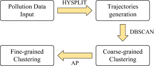
Air pollution prediction with machine learning: a case study of Indian cities

A quantitative assessment of natural and anthropogenic effects on the occurrence of high air pollution loading in Dhaka and neighboring cities and health consequences

Air pollution and its health impacts in Malaysia: a review

Xu, X., Yang, H., Li, C.: Theoretical model and actual characteristics of air pollution affecting health cost: a review. Int. J. Environ. Res. Public Health (2022). https://doi.org/10.3390/ijerph19063532

Article   Google Scholar  

Pandya, S., Gadekallu, T.R., Maddikunta, P.K.R., Sharma, R.: A study of the impacts of air pollution on the agricultural community and yield crops (indian context). Sustainability (2022). https://doi.org/10.3390/su142013098

Bachechi, C., Po, L., Rollo, F.: Big data analytics and visualization in traffic monitoring. Big Data Res. 27 , 100292 (2022). https://doi.org/10.1016/j.bdr.2021.100292

Blázquez-García, A., Conde, A., Mori, U., Lozano, J.A.: A review on outlier/anomaly detection in time series data. ACM Comput. Surv. (2021). https://doi.org/10.1145/3444690

Guo, Y., Guo, S., Jin, Z., Kaul, S., Gotz, D., Cao, N.: Survey on visual analysis of event sequence data. IEEE Trans. Vis. Comput. Graph. 28 (12), 5091–5112 (2022). https://doi.org/10.1109/TVCG.2021.3100413

Taylor, G.I.: I. eddy motion in the atmosphere. Philos. Trans. R. Soc. Lond. Ser. A Contain. Pap. Math. Phys. Character 215 (523-537), 1–26 (1915). https://doi.org/10.1098/rsta.1915.0001

Taylor, G.I.: Diffusion by continuous movements. Proc. Lond. Math. Soc. 2 (1), 196–212 (1922). https://doi.org/10.1112/plms/s2-20.1.196

Article   MathSciNet   MATH   Google Scholar  

Liu, Y., Wang, T.: Worsening urban ozone pollution in china from 2013 to 2017—part 2: the effects of emission changes and implications for multi-pollutant control. Atmos. Chem. Phys. 20 (11), 6323–6337 (2020). https://doi.org/10.5194/acp-20-6323-2020

Dong, Z., Wang, S., Xing, J., Chang, X., Ding, D., Zheng, H.: Regional transport in beijing-tianjin-hebei region and its changes during 2014–2017: the impacts of meteorology and emission reduction. Sci. Total Environ. 737 , 139792 (2020). https://doi.org/10.1016/j.scitotenv.2020.139792

Ballesteros-González, K., Sullivan, A.P., Morales-Betancourt, R.: Estimating the air quality and health impacts of biomass burning in northern south America using a chemical transport model. Sci. Total Environ. 739 , 139755 (2020). https://doi.org/10.1016/j.scitotenv.2020.139755

Vander Hoorn, S., Johnson, J.S., Murray, K., Smit, R., Heyworth, J., Lam, S., Cope, M.: Emulation of a chemical transport model to assess air quality under future emission scenarios for the southwest of western australia. Atmosphere (2022). https://doi.org/10.3390/atmos13122009

Tao, H., Xing, J., Pan, G., Pleim, J., Ran, L., Wang, S., Chang, X., Li, G., Chen, F., Li, J.: Impact of anthropogenic heat emissions on meteorological parameters and air quality in Beijing using a high-resolution model simulation. Front. Environ. Sci. Eng. 16 (4), 1–11 (2022). https://doi.org/10.1007/s11783-021-1478-3

Kim, M.: Visualization of dynamic network evolution with quantification of node attributes. IEEE Trans. Netw. Sci. Eng. 8 (3), 2316–2325 (2021). https://doi.org/10.1109/TNSE.2021.3087334

Article   MathSciNet   Google Scholar  

Feng, Z., Li, H., Zeng, W., Yang, S.-H., Qu, H.: Topology density map for urban data visualization and analysis. IEEE Trans. Vis. Comput. Graph. 27 (2), 828–838 (2021). https://doi.org/10.1109/TVCG.2020.3030469

Linhares, C.D., Ponciano, J.R., Paiva, J.G.S., Travençolo, B.A., Rocha, L.E.: A comparative analysis for visualizing the temporal evolution of contact networks: a user study. J. Vis. 24 (5), 1011–1031 (2021). https://doi.org/10.1007/s12650-021-00759-x

Meidiana, A., Hong, S.-H., Eades, P.: New quality metrics for dynamic graph drawing. In: International Symposium on Graph Drawing and Network Visualization, pp. 450–465 (2020). https://doi.org/10.1007/978-3-030-68766-3_35

Ponciano, J.R., Linhares, C.D.G., Rocha, L.E.C., Faria, E.R., Travençolo, B.A.N.: Combining clutter reduction methods for temporal network visualization. In: Proceedings of the 37th ACM/SIGAPP Symposium on Applied Computing. SAC ’22, pp. 1748–1755. Association for Computing Machinery, New York, NY, USA (2022). https://doi.org/10.1145/3477314.3507018

Liu, Z., Huang, C., Yu, Y., Dong, J.: Motif-preserving dynamic attributed network embedding. In: Proceedings of the Web Conference 2021. WWW ’21, pp. 1629–1638. Association for Computing Machinery, New York, NY, USA (2021). https://doi.org/10.1145/3442381.3449821

Sabarish, B.A., Karthi, R., Kumar, T.G.: Graph similarity-based hierarchical clustering of trajectory data. Procedia Comput. Sci. 171 , 32–41 (2020). https://doi.org/10.1016/j.procs.2020.04.004

Feng, K., Wang, P., Wu, J., Wang, W.: L-match: a lightweight and effective subsequence matching approach. IEEE Access 8 , 71572–71583 (2020). https://doi.org/10.1109/ACCESS.2020.2987761

Fernandez, I., Manglik, A., Giannoula, C., Quislant, R., Mansouri Ghiasi, N., Gómez-Luna, J., Gutierrez, E., Plata, O., Mutlu, O.: Accelerating Time Series Analysis via Processing using Non-Volatile Memories. arXiv e-prints (2022) https://doi.org/10.48550/arXiv.2211.04369

Li, Z., Guo, J., Li, H., Wu, T., Mao, S., Nie, F.: Speed Up Similarity Search of Time Series Under Dynamic Time Warping, vol. 7, pp. 163644–163653 (2019). https://doi.org/10.1109/ACCESS.2019.2949838

Rakthanmanon, T., Campana, B., Mueen, A., Batista, G., Westover, B., Zhu, Q., Zakaria, J., Keogh, E.: Searching and mining trillions of time series subsequences under dynamic time warping. KDD ’12, pp. 262–270. Association for Computing Machinery, New York, NY, USA (2012). https://doi.org/10.1145/2339530.2339576

Linardi, M., Palpanas, T.: Scalable data series subsequence matching with ulisse. VLDB J. 29 (6), 1449–1474 (2020). https://doi.org/10.1007/s00778-020-00619-4

Barandas, M., Folgado, D., Fernandes, L., Santos, S., Abreu, M., Bota, P., Liu, H., Schultz, T., Gamboa, H.: Tsfel: time series feature extraction library. SoftwareX 11 , 100456 (2020). https://doi.org/10.1016/j.softx.2020.100456

Gao, J., Song, X., Wen, Q., Wang, P., Sun, L., Xu, H.: RobustTAD: Robust Time Series Anomaly Detection via Decomposition and Convolutional Neural Networks. arXiv e-prints (2020) https://doi.org/10.48550/arXiv.2002.09545 arXiv:2002.09545

Ceci, M., Corizzo, R., Japkowicz, N., Mignone, P., Pio, G.: Echad: embedding-based change detection from multivariate time series in smart grids. IEEE Access 8 , 156053–156066 (2020). https://doi.org/10.1109/ACCESS.2020.3019095

Boniol, P., Palpanas, T.: Series2Graph: Graph-based Subsequence Anomaly Detection for Time Series. arXiv e-prints, pp. 2207–12208 (2022) https://doi.org/10.48550/arXiv.2207.12208

Liu, D., Veeramachaneni, K., Geiger, A., Li, V.O.K., Qu, H.: AQEyes: Visual Analytics for Anomaly Detection and Examination of Air Quality Data. arXiv e-prints (2021) https://doi.org/10.48550/arXiv.2103.12910

Deng, Z., Weng, D., Chen, J., Liu, R., Wang, Z., Bao, J., Zheng, Y., Wu, Y.: Airvis: visual analytics of air pollution propagation. IEEE Trans. Vis. Comput. Graph. 26 (1), 800–810 (2020). https://doi.org/10.1109/TVCG.2019.2934670

Lu, W., Ai, T., Zhang, X., He, Y.: An interactive web mapping visualization of urban air quality monitoring data of china. Atmosphere (2017). https://doi.org/10.3390/atmos8080148

Kalo, M., Zhou, X., Li, L., Tong, W., Piltner, R.: Chapter 8—sensing air quality: spatiotemporal interpolation and visualization of real-time air pollution data for the contiguous united states, pp. 169–196 (2020). https://doi.org/10.1016/B978-0-12-815822-7.00008-X

Qu, D., Lin, X., Ren, K., Liu, Q., Zhang, H.: Airexplorer: visual exploration of air quality data based on time-series querying. J. Vis. 23 (6), 1129–1145 (2020). https://doi.org/10.1007/s12650-020-00683-6

Chen, P.: Visualization of real-time monitoring datagraphic of urban environmental quality. Eurasip J. Image Video Process. 2019 (1), 1–9 (2019). https://doi.org/10.1186/s13640-019-0443-6

Yang, X., Peng, H., Zhang, Q.: Visual analysis of heterogenous air pollution data. In: Proceedings of the 4th International Conference on Computer Science and Software Engineering. CSSE ’21, pp. 300–306. Association for Computing Machinery, New York, NY, USA (2021). https://doi.org/10.1145/3494885.3494940

Kong, L., Tang, X., Zhu, J., Wang, Z., Li, J., Wu, H., Wu, Q., Chen, H., Zhu, L., Wang, W., Liu, B., Wang, Q., Chen, D., Pan, Y., Song, T., Li, F., Zheng, H., Jia, G., Lu, M., Wu, L., Carmichael, G.R.: A 6-year-long (2013–2018) high-resolution air quality reanalysis dataset in china based on the assimilation of surface observations from cnemc. Earth Syst. Sci. Data 13 (2), 529–570 (2021). https://doi.org/10.5194/essd-13-529-2021

Jooybari, S.A., Peyrowan, H., Rezaee, P., Gholami, H.: Evaluation of pollution indices, health hazards and source identification of heavy metal in dust particles and storm trajectory simulation using hysplit model (case study: Hendijan center dust, southwest of iran). Environ. Monit. Assess. 194 (2), 107 (2022). https://doi.org/10.1007/s10661-022-09760-9

Zaib, S., Lu, J., Bilal, M.: Spatio-temporal characteristics of air quality index (aqi) over northwest china. Atmosphere (2022). https://doi.org/10.3390/atmos13030375

Ouyang, T., Shen, X.: Online structural clustering based on dbscan extension with granular descriptors. Inf. Sci. 607 , 688–704 (2022). https://doi.org/10.1016/j.ins.2022.06.027

Chen, J., Chen, B.: Development of driving cycle for light vehicle based on the ap clustering method. In: Computational and Experimental Simulations in Engineering: Proceedings of ICCES 2020, vol. 2, pp. 495–506 (2021). https://doi.org/10.1007/978-3-030-67090-0_40

Chatzigeorgakidis, G., Skoutas, D., Patroumpas, K., Athanasiou, S., Skiadopoulos, S.: Indexing geolocated time series data. In: Proceedings of the 25th ACM SIGSPATIAL International Conference on Advances in Geographic Information Systems. SIGSPATIAL ’17. Association for Computing Machinery, New York, NY, USA (2017). https://doi.org/10.1145/3139958.3140003

Wen, M., Ma, Y., Zhang, W., Tian, Y., Wang, Y.: High-resolution load profile clustering approach based on dynamic largest triangle three buckets and multiscale dynamic warping path under limited warping path length. J. Mod. Power Syst. Clean Energy (2022). https://doi.org/10.35833/MPCE.2022.000386

Download references

Acknowledgements

This work was partially supported by the National Key R &D Program of China under Grand No. 2021YFE0108400 and partly supported by the National Natural Science Foundation of China under Grant No. 62172294.

Author information

Authors and affiliations.

College of Intelligence and Computing, Tianjin University, Tianjin, 300350, China

Jiayang Li & Chongke Bi

You can also search for this author in PubMed   Google Scholar

Corresponding author

Correspondence to Chongke Bi .

Additional information

Publisher's note.

Springer Nature remains neutral with regard to jurisdictional claims in published maps and institutional affiliations.

Rights and permissions

Springer Nature or its licensor (e.g. a society or other partner) holds exclusive rights to this article under a publishing agreement with the author(s) or other rightsholder(s); author self-archiving of the accepted manuscript version of this article is solely governed by the terms of such publishing agreement and applicable law.

Reprints and permissions

About this article

Li, J., Bi, C. Visual analysis of air pollution spatio-temporal patterns. Vis Comput 39 , 3715–3726 (2023). https://doi.org/10.1007/s00371-023-02961-4

Download citation

Accepted : 09 June 2023

Published : 24 June 2023

Issue Date : August 2023

DOI : https://doi.org/10.1007/s00371-023-02961-4

Share this article

Anyone you share the following link with will be able to read this content:

Sorry, a shareable link is not currently available for this article.

Provided by the Springer Nature SharedIt content-sharing initiative

• Air pollution
• Transport pattern
• Sketch match
• Visual analysis
• Find a journal
• Publish with us
• Track your research

• Open access
• Published: 12 February 2019

Visualization of real-time monitoring datagraphic of urban environmental quality

• Pengyu Chen   ORCID: orcid.org/0000-0003-2383-2881 1  

EURASIP Journal on Image and Video Processing volume  2019 , Article number:  42 ( 2019 ) Cite this article

9370 Accesses

42 Citations

2 Altmetric

Metrics details

Quality of urban environment directly affects people health, and it is important to understand the real-time status of urban air quality. Air quality monitoring, data analysis, and visualization can grasp the concentration data of air pollutants in cities. In view of the current air quality monitoring using digital displays, it is difficult for users to intuitively determine the air pollution level with unsatisfied interaction mode of the data query. Using the real-time monitoring data of 23 observation points in Beijing, the work based on Google Earth applied Keyhole Markup Language (KML) for the visualization of air monitoring data. The interactive query makes it easier for users to query air quality, and gradually varied color can visually highlight the air quality level. Visualization of data has stronger expression (more images and more intuitive) than the original data table, which is beneficial for further analysis of data.

1 Introduction

The quality of the urban environment is related to the health of urban residents. Under global warming and urbanization, population concentration is getting higher and higher, with urban environmental quality becoming prominent. The coordinated development of human settlements and urbanization has become the focus in the world. At 2017 World Climate Conference in Copenhagen, members, focusing on energy conservation and emission reduction as well as the ecology and low carbon development, signed the Copenhagen Accord [ 1 ].

At present, most cities have established the complete monitoring system for environmental quality to measure six parameters (PM2.5, PM10, SO2, NO2, CO, O3) of air quality index (AQI), wind direction, noise, temperature and humidity, negative oxygen ions, and light, wherein AQI is the focus of real-time monitoring, especially for PM2.5 and PM10, because respirable particulate matter is a typical carcinogen. Urban air pollution leads to an increase in cancer incidence, and people can reduce outdoor activities due to air pollution. Real-time monitoring of air quality has the advantages such as guiding the travel of residents, regulating urban infrastructure traffic, strengthening medical care for respiratory diseases, and insisting environmental protection departments for reducing/stopping production of pollution-emitting enterprises.

As early as 1996, China formulated Ambient Air Quality Standard , which details the classification of urban air quality, standard classification, major pollutants, and their concentration limits at various levels. At present, China’s industry is still a traditional energy consumption structure. For economic development, a large amount of petrochemical energy such as coal and oil is consumed every year, causing serious pollution to the air. In winter in the north, extreme foggy weather appears due to heating, which leads to school suspension, factory shutdowns, and traffic control. It is the basis for improving urban air quality and the guarantee for the health of the masses by integrating computer network, air quality sensing, and data visualization into an urban air quality monitoring system.

Advances in current sensor technology and Internet of Things technology have made it possible to monitor air quality in various areas of the city in real time. However, the large amount of data collected in real time brings inconvenience to analysis and processing. Explosively growing big data sometimes exceeds the processing power of the system, and existing data mining techniques only use the tip of the iceberg [ 2 ]. Data visualization can transform data into intuitive graphical images and provide interaction and analysis between the server and users, showing the valuable rules between complex and massive data [ 3 ]. Data visualization is used to integrate the high-bandwidth, high-speed, and large-capacity storage vision system with the computer system of powerful computing and logic judgment. The graphic visualization of real-time data of urban air quality displays the air quality data obtained by real-time monitoring, enabling users to efficiently capture hidden features and patterns in big data. Without efficient datagraphic visualization analysis, it is impossible to achieve good management of urban air quality.

Based on Google Earth, the work proposed a graphical visualization method for real-time monitoring data of urban air quality, which is helpful to grasp the change and development trends of urban air quality and control pollution. It has theoretical significance and practical value for environmental management and public services.

2 Methods for visualized analysis

2.1 visualized analysis of air quality data.

There are a number of visualization methods available for analysis and processing of air quality data with one or more visualization tools. Qu et al. [ 4 ] used S-shaped parallel coordinates, a weighting map, and a polar coordinate system embedded in circular pixel strips to analyze the fog and haze of Hong Kong. Li et al. [ 5 ] used a multi-dimensional view to analyze air quality and meteorological data. A correlation detection view is proposed to visualize the change of air quality. Liao et al. [ 6 ] used the networked visualized analysis system to monitor air quality data in Beijing, with Geographical Information System (GIS), parallel coordinate, and splattering. Li et al. [ 7 ] analyzed the air pollution data in Beijing and used a two-dimensional diagram for the pollution levels of areas. Visualization for data analysis is difficult for ordinary users to understand, because the two-dimensional diagram of the data often fails to meet the growing demands of air quality information systems. Data should be presented in an interesting and easy-to-understand format to deliver information to end users.

In 2010, Canadian researches Aaron Van Daniela and Randall Martin added the total amount of aerosols monitored by NASA (National Aeronautics and Space Administration) satellites and superimposed them on the vertical distribution of aerosols calculated by computer models to obtain the global image of PM2.5 concentration distribution. PM2.5 pollution in China is very serious, and Shandong Province in China is the most polluted area of PM2.5 in the world. There is a common flaw in most of these traditional data visualization methods—they separate the relationship between air quality and time and space and statically calculate air quality data in the past. It cannot display air quality dynamically in real time, with no good predictability of future air quality.

2.2 Google Earth-based visualization system

Google Earth is a virtual Earth software developed by Google Inc., which arranges satellite photos, aerial photography, and GIS on a three-dimensional model of the Earth. Users can view high-definition satellite images from the world for free through the client software of Google Earth. The satellite images, not from a single data source, are the data fusion of satellite imagery and aerial imagery.

Charts are represented in a fixed scene in traditional air quality visualization methods and cannot be dynamically updated based on changes in location and real-time data. However, to master the air quality of a single city or a group of cities, it is impossible to rely on static charts without user interaction. The air quality of a city exists under specific time and space, and the charts are meaningless if it is deviating from geographical location and observation time.

Using Google Earth to visualize urban air quality combines air quality information with time and space. It visualizes massive amounts of air quality data in an intuitive and vivid way, breaking traditional patterns of data, formulas, and charts that express air quality. The simulation on the 3D virtual Earth platform can obtain the dynamic change of air quality to enhance the authenticity of data visualization of air quality. It is easy for users to understand and conducive to providing decision support for public management and improving urban air quality.

Figure  1 shows the average PM2.5 air quality index of monthly and weekly hotlist in the traditional table. Figure  2 shows the design sketch of data visualization based on Google Earth. From the comparison, the use of Google Earth to achieve data visualization of air quality is more intuitive and provides more images.

Average PM2.5 air quality index of monthly and weekly hotlist in the traditional table

Design sketch of data visualization based on Google Earth

At present, many scholars have performed lots of useful work in this field. Environmental information is integrated into Google Earth [ 8 ], and visual dynamic playback of pollution distribution is implemented based on Google Earth [ 9 ]. Urban air pollution is investigated by Google Earth with detailed explanation [ 10 ]. Google Earth is applied to the simulation of urban air pollution spread. Based on the distribution of atmospheric pollution concentration, dangerous areas are drawn in the urban map of Google Earth, providing the basis for emergency decision-making [ 11 ]. The data of 3D scanning lidar is integrated into Google Earth to observe real-time atmospheric pollution. The visualization of information can quickly determine the location of pollution sources and assess which areas are seriously affected [ 12 ].

3 Data visualization of urban air quality

3.1 keyhole markup language (kml).

KML is a markup language based on XML standard, which uses a markup structure with nested elements and attributes to express geotagging. KML files are written according to the KML language, widely used in software such as Google Earth, Google Map, and Google Maps for mobile [ 13 ]. The basic structure of a KML file is shown in a KML code, which uses a yellow pushpin to mark a location on the surface of the Earth. Place mark is the most commonly used geographic feature in Google Earth.

KML files are used to exchange geographic data in Google Earth. File-based data exchange has been one of the main ways of software data exchange. KML files define a number of TAGS used to specify how geographic data is displayed. Geographic features that can be defined include locations, descriptions, overlays, paths, and polygons.

3.2 Public data of air quality

With the rapid development of Internet technology, local government agencies provide public data on air quality monitoring to protect the health of the people. USA, Britain, Australia, and Canada have operated public data sites. For example, the US AirNow website specializes in providing air quality data and its impact on human health, helping people to make healthy behaviors based on different air quality [ 14 ]. UK Air Quality Archive is the UK’s authoritative platform of air quality query. The Chinese government has also established numerous public data sites. However, regarding air pollution data, the public generally obtains data from the mass media. Since numerical data is difficult to understand, it is necessary to visualize the data.

The work studied Beijing, which is located at 39″ 26′ to 41″ 03′ north latitude and 115″ 25′ to 117″ 30′ east longitude on the northwestern edge of the North China Plain with a total area of 164.1 thousand square kilometers and an urban area of 1401 thousand square kilometers. The west, north, and northeast of Beijing are surrounded by mountains, and the southeast is a large plain that slowly slopes towards the Bohai Sea. The altitude of the Beijing Plain is 20 to 60 m, and the mountain is generally 1000 to 1500 m above the sea level.

The real-time monitoring data of air quality in the work comes from the Beijing Municipal Environmental Monitoring Center established in 1974. The center is the first-level station of national environmental monitoring that provides environmental quality monitoring of environmental factors (such as atmosphere, water, noise, soil, and ecology), the monitoring of pollution sources, and the emergency monitoring of sudden pollution accidents in Beijing. Figure  3 shows the distribution of environmental assessment points in 23 districts across Beijing. The website’s data is updated every half hour, and the data of urban air quality can be obtained by the Web Service interface. Table  1 shows the specific parameters and sample data of air quality data in the work. The data also includes other information such as weather forecast, wind direction, typhoon, and monitoring station. Only air pollution data is used in the work.

In Table  1 , AQI represents air quality index with no unit in the range of 0–500, O 3 /8 h the average concentration of ozone within 8 h, PM2.5 the particles with a diameter of less than 2.5 μm, and PM10 the particles with a diameter of less than 10 μm.

Distribution of 23 air quality observation points in Beijing

3.3 Visualization process of air quality data

To improve the intuitiveness of air quality data, the work implemented data visualization of air quality based on Google Earth and KML. The real-time monitoring data of air quality was obtained from the Beijing Municipal Environmental Monitoring Center, stored in the server with regular update. By developing and applying the KML Generator program, the Web Service was used to request air quality data from the server and visualize the data by Google Earth. The generated KML code and its URL were stored in the public folder of Dropbox. They were linked to Google Earth via KML network links that read air quality data in the server in real time [ 15 , 16 , 17 ]. Once the server is properly configured with the shared URL of KML files, users who have installed Google Earth can view KML files hosted in the public web server. Figure  4 shows the specific process of reading data and visualizing air quality data using KML files.

Process of reading air quality data and data visualization

The KML code for real-time visualization of air quality using KML network link is shown below. The data in the server is read periodically, with the display refreshed at a specified time interval [ 18 , 19 ].

3.4 KML Generator program

KML Generator program requests the server to read the air quality data through the longitude and latitude of each observation point. Figure  5 shows the structure of KML files generated after obtaining the data. Each observation point corresponds to a folder containing <name>, <description>, and six <Placemark> tags. <name> indicates the name of the observation point, <description> shows a brief description of the observation area, and six <Placemark> corresponds to six kinds of polluting gases (including names and short descriptions). <Style> label indicates the color of each contaminant. The transparency of color depends on the level of contamination in the observation area—the darker color means the higher level of contamination.

KML structure for visualization of the pollution level in the observation area

3.5 Visualization of air quality

Figure  6 shows the visualization of air pollution data using KML and Google Earth. In the distribution of AQI, red indicates the high concentration of air pollutants, and blue the low concentration. The air pollution concentration is low in the north and high in the south, which is consistent with the geographical environment of Beijing. Forested land and orchards are mainly in the northern mountain areas of Beijing, with less settlements, factories, and roads. The south-central part is a bustling and crowed urban area with dense personnel and vehicles, resulting in a significantly lower air quality than the north. For the distribution of specific pollutants such as PM2.5, PM10, SO2, and NO2, users can switch to the single-pollutant distribution mode by clicking the label. The visualization in Fig.  6 can only show the overall air quality. More specific visualization results can be obtained by the interactive query in Google Earth.

Average AQI heat map in Beijing

4 Results and discussion

Visual interactive query allows users to learn more specific air quality values, performing a series of selection operations through the interactive graphical interface to query. Users intuitively transmit the query without complex query statements. The data shorted in the server can be directly read and written into KML format recognized by Google Earth [ 20 , 21 , 22 ]. The template changes according to different needs, and the air quality data is displayed in Google Earth with various forms.

Figure  7 shows the real-time AQI query for the area around Shunyi New City observation point. Users simply click on the observation point indicated by the red arrow in the graph to pop up the query results. In general, the size of the display screen is limited. To make users focus on a certain detail while browsing Google Earth, animation or a pop-up window (used in the work) is required to attract users’ attention.

Interactive query of air quality

To show the dynamic change process of the AQI in the past 24 h, a histogram is used to combine the cylinders of different colors to represent the AQI value. The green cylinder indicates the air quality level is excellent, with an AQI value between 0 and 50. The yellow one indicates the air quality level is good, with an AQI value between 0 and 50. The deepest purple indicates the air quality is severely polluted, with an AQI value greater than 300. For each air quality level, the effects of air on human health and recommended actions are briefly introduced. In this way, the overall understanding of Fig.  6 can be gradually refined to understand the specific air quality of each area.

Figure  8 shows the variation of contaminants within 24 h—six pollutants, temperature, pressure, and humidity. The horizontal axis in the bar chart is the time axis, indicating the last 48 h from now. The vertical axis represents the parameter values. On the far right is the actual value range of the parameter value within 48 h, not the theoretical value range of the parameter. The higher the cylinder height, the closer the parameter value is to the maximum value. The colors of the cylinder further distinguish different parameter values. As the color changes, the corresponding parameter value gradually becomes large. It shows the changes in air quality over the past period of time, and a rough estimate can be made accordingly on the concentration of each pollutant over a period of time. After the analysis process of more data, the laws implied in the big data make the air quality data more valuable.

Multiple air quality parameters

5 Conclusions

With the development of social economy, a large amount of harmful substances generated by industrial production and automobile exhaust gas are discharged into the air, causing serious air pollution. It is the most serious environmental problem facing most industrial cities in the world. Taking Beijing as an example, the work used the real-time monitoring data of 23 observation points throughout the city to visualize the monitoring data in the Google Earth. Users can understand the air quality distribution from a macro perspective or obtain the specific air quality data by the interactive query to understand the time trends of air pollution, pollutants, and air quality levels in different regions at different times.

In the future work, it is necessary to study the cloud storage for the data of each observation point, the storage of more data in a lone time range, and the acquisition of complete data information for further analysis and utilization of data. On the other hand, the reasonable air quality prediction model with big data will be studied to predict the air quality, thus meeting the needs of the public.

Abbreviations

• Air quality index

Geographical Information System

Keyhole Markup Language

National Aeronautics and Space Administration

Doniger D (2009) The Copenhagen Accord: a big step forward, NRDC Climate Center. Accessed 21 Dec 2009

Google Scholar  

H. Mayer, J. Holst, D. Schindler, D. Ahrens, Evolution of the air pollution in SW Germany evaluated by the long-term air quality index LAQx. Atmos. Environ. 42 (20), 5071–5078 (2008)

Article   Google Scholar  

Sarkar, D. (2008). Lattice: multivariate data visualization with R. Springer Science & Business Media

H. Qu, W.Y. Chan, A. Xu, K.L. Chung, K.H. Lau, P. Guo, Visual analysis of the air pollution problem in Hong Kong. IEEE Trans. Vis. Comput. Graph. 13 (6), 1408–1415 (2007)

J. Li, Z. Xiao, H.Q. Zhao, Z.P. Meng, K. Zhang, Visual analytics of smogs in China. J. Vis. 19 (3), 461–474 (2016)

Z. Liao, Y. Peng, Y. Li, X. Liang, Y. Zhao. A web-based visual analytics system for air quality monitoring data, 2014 22nd International Conference on Geoinformatics, Kaohsiung, The Institute of Electrical and Electronics Engineers, INC. 1-6 (Piscataway, NJ, 2014)

H. Li, H. Fan, F. Mao, A visualization approach to air pollution data exploration—a case study of air quality index (PM2. 5) in Beijing, China. Atmosphere 7 (3), 35 (2016)

N. Kussul, A. Shelestov, S. Skakun, Grid and sensor web technologies for environmental monitoring. Earth Sci. Inf. 2 (1–2), 37–51 (2009)

R. Varatharajan, G. Manogaran, M.K. Priyan, V.E. Balaş, C. Barna, Visual analysis of geospatial habitat suitability model based on inverse distance weighting with paired comparison analysis. Multimed. Tools Appl. 77 (14), 17573–17593 (2018)

M.J. URBAN, in 2009 Portland GSA Annual Meeting . Using Google Earth to examine metropolitan air pollution (2009)

Y. CHU, D. LIANG, J. GUO, X. FENG, J. FANG, Y. CHEN, Z. ZHANG, Z. YIN, Analysis of urban air pollution diffusion simulation based on Google Earth. Ind. Saf. Environ. Prot. 40 (09), 36–39 (2014)

C. Chiang, J. Nee, S. Das, S. Sun, Y. Hsu, H. Chiang, et al., in AGU Fall Meeting Abstracts . Incorporation of 3-D scanning lidar data into Google Earth for real-time air pollution observation (2011)

M. Silberbauer, W. Geldenhuys, in Academic track of the 2008 Free and Open Source Software for Geospatial (FOSS4G) Conference, incorporating the GISSA 2008 Conference, Cape Town, South Africa . Using keyhole markup language to create a spatial interface to South African water resource data through Google Earth (2008)

T. LU, Application of AIRNow ambient air quality notification system of USA in Shanghai. Environ. Monit. Forewarning 3 (01), 4–7 (2011)

S. Tavani, P. Granado, A. Corradetti, et al., Building a virtual outcrop, extracting geological information from it, and sharing the results in Google Earth via OpenPlot and Photoscan: an example from the Khaviz Anticline (Iran). Comput. Geosci. 63 , 44–53 (2014)

A. Chen, G. Leptoukh, S. Kempler, C. Lynnes, A. Savtchenko, D. Nadeau, J. Farley, Visualization of A-Train vertical profiles using Google Earth. Comput. Geosci. 35 (2), 419–427 (2009)

A. Triantafyllou, A. Watlet, C. Bastin, Geolokit: an interactive tool for visualising and exploring geoscientific data in Google Earth. Int. J. Appl. Earth Obs. Geoinf. 62 , 39–46 (2017)

Q. Zhou, Multi-layer affective computing model based on emotional psychology. Electron. Commer. Res. 18 (1), 109–124 (2018)

Q. Zhou, J. Luo, The study on evaluation method of urban network security in the big data era. Intell. Autom. Soft Comput. 24 (1), 133–138 (2018)

M. Richards, M. Ghanem, M. Osmond, Y. Guo, J. Hassard, Grid-based analysis of air pollution data. Ecol. Model. 194 (1–3), 274–286 (2006)

D. Christin, A. Reinhardt, S.S. Kanhere, M. Hollick, A survey on privacy in mobile participatory sensing applications. J. Syst. Softw. 84 (11), 1928–1946 (2011)

E. Kanjo, Noisespy: a real-time mobile phone platform for urban noise monitoring and mapping. Mob. Netw. Appl. 15 (4), 562–574 (2010)

Download references

Acknowledgements

Thank for the editor and reviewers.

No funding was received.

Availability of data and materials

Data will not be shared; reason for not sharing the data and materials is that the work submitted for review is not completed. The research is still ongoing, and those data and materials are still required by my team for further investigations.

Author information

Authors and affiliations.

Northwest University, Xi’an, 710127, China

Pengyu Chen

You can also search for this author in PubMed   Google Scholar

Contributions

PC designed the research, analyzed the data, and wrote and edited the manuscript. The author read and approved the final manuscript.

Corresponding author

Correspondence to Pengyu Chen .

Ethics declarations

Ethics approval and consent to participate.

I approved.

Consent for publication

Competing interests.

The author declares that he has no competing interests. He has seen the manuscript and approved its submission to the journal. The author confirmed that the content of the manuscript has not been published or submitted for publication elsewhere.

Publisher’s Note

Springer Nature remains neutral with regard to jurisdictional claims in published maps and institutional affiliations.

Rights and permissions

Open Access This article is distributed under the terms of the Creative Commons Attribution 4.0 International License ( http://creativecommons.org/licenses/by/4.0/ ), which permits unrestricted use, distribution, and reproduction in any medium, provided you give appropriate credit to the original author(s) and the source, provide a link to the Creative Commons license, and indicate if changes were made.

Reprints and permissions

About this article

Cite this article.

Chen, P. Visualization of real-time monitoring datagraphic of urban environmental quality. J Image Video Proc. 2019 , 42 (2019). https://doi.org/10.1186/s13640-019-0443-6

Download citation

Received : 18 September 2018

Accepted : 04 February 2019

Published : 12 February 2019

DOI : https://doi.org/10.1186/s13640-019-0443-6

Share this article

Anyone you share the following link with will be able to read this content:

Sorry, a shareable link is not currently available for this article.

Provided by the Springer Nature SharedIt content-sharing initiative

• Data visualization
• Google Earth
• Air pollution

Analysis of Air Pollution Data in India between 2015 and 2019

1 Center for Policy Research on Energy and Environment, School of Public and International Affairs, Princeton University, Princeton, NJ 08544, USA 2 Department of Civil and Environmental Engineering, Princeton University, Princeton, NJ 08544, USA

  Copyright  The Author(s). This is an open access article distributed under the terms of the  Creative Commons Attribution License (CC BY 4.0) , which permits unrestricted use, distribution, and reproduction in any medium, provided the original author and source are cited.

• Download: PDF | Supplemental Material

Sharma, D., Mauzerall, D. (2022). Analysis of Air Pollution Data in India between 2015 and 2019. Aerosol Air Qual. Res. 22, 210204. https://doi.org/10.4209/aaqr.210204

• Analysis of PM 10 , PM 2.5 , SO 2 , NO 2 and O 3 measurements across India from 2015–2019.
• First comprehensive analysis of Indian government and US Air-Now data.
• More national ambient air quality standard exceedances in north than south India.
• Provides baseline for evaluation of mitigation measures and atmospheric models.

India suffers from among the worst air pollution in the world. In response, a large government effort to increase air quality monitoring is underway. We present the first comprehensive analysis of government air quality observations from 2015–2019 for PM 10 , PM 2.5 , SO 2 , NO 2 and O 3 from the Central Pollution Control Board (CPCB) Continuous Ambient Air Quality Monitoring (CAAQM) network and the manual National Air Quality Monitoring Program (NAMP), as well as PM 2.5 from the US Air-Now network. We address inconsistencies and data gaps in datasets using a rigorous procedure to ensure data representativeness. We find particulate pollution dominates the pollution mix across India with virtually all sites in northern India (divided at 23.5°N) exceeding the annual average PM 10 and PM 2.5 residential national ambient air quality standards (NAAQS) by 150% and 100% respectively, and in southern India exceeding the PM 10 standard by 50% and the PM 2.5 standard by 40%. Annual average SO 2 , NO 2 and MDA8 O 3 generally meet the residential NAAQS across India. Northern India has (~10%–130%) higher concentrations of all pollutants than southern India, with only SO 2 having similar concentrations. Although inter-annual variability exists, we found no significant trend of these pollutants over the five-year period. In the five cities with Air-Now PM 2.5 measurements - Delhi, Kolkata, Mumbai, Hyderabad and Chennai, there is reasonable agreement with CPCB data. The PM 2.5 CPCB CAAQM data compares well with satellite derived annual surface PM 2.5 concentrations (Hammer et al. , 2020), with the exception of the western desert region prior to 2018 when surface measurements exceeded satellite retrievals. Our reanalyzed dataset is useful for evaluation of Indian air quality from satellite data, atmospheric models, and low-cost sensors. Our dataset also provides a baseline to evaluate the future success of National Clean Air Programme as well as aids in assessment of existing and future air pollution mitigation policies.

Keywords: Air pollution, India, surface observations, CPCB, continuous and manual data, US AirNow

1 INTRODUCTION

Concerns over poor air quality in India have increased over the past few years with increasing evidence of the adverse impacts on health (Balakrishnan   et al. , 2014; Chowdhury and Dey, 2016; Balakrishnan   et al. , 2019), agricultural yields (Avnery   et al. , 2011, 2013; Ghude   et al. , 2014; Gao   et al. , 2020) and the economy (Pandey   et al. , 2021). Rapid growth and industrialization in India have resulted in some of the most polluted air in the world. Projections forecast further decreases in air quality and a 24% increase in PM 2.5   associated premature mortalities by 2050 relative to 2015 (GBD MAPS Working Group, 2018; Brauer   et al. , 2019). According to recent estimates based on the Global Exposure Mortality Model (GEMM), total premature mortality due to ambient PM 2.5   exposure in India increased approximately 47% between 2000 and 2015 (Chowdhury   et al. , 2020). Surface O 3   concentrations are also likely to increase with growing industrial emissions and increasing temperatures due to climate change resulting in additional stress on agricultural yields and public health (Avnery   et al. , 2011; Silva   et al. , 2017).

India has a national ambient surface monitoring network that started in 1987 and has become more extensive over time with a substantial increase in the number and spatial extent of continuous and manual monitoring stations between 2015 and 2019. At present, the Central Pollution Control Board (CPCB), along with the State Pollution Control Boards (SPCBs), run the most extensive monitoring network in the country under the National Air Quality Monitoring Program (NAMP). As of 2019, NAMP cooperatively operated (with CPCB and SPCBs) over 750 manual monitoring stations (compared with 20 in 1987 when monitoring first began and 450 in 2015 when our analysis starts) which publicly archive annual average concentrations of PM 10 , PM 2.5 , SO 2   and NO 2   ( https://cpcb.nic.in/namp-data/ ). As of 2019, over 220 Continuous Ambient Air Quality Monitoring (CAAQM) stations operated (compared with less than 50 stations in 2015 when our analysis starts). CPCB archives publicly available, real time data, every 15 minutes, from over 220 stations across India of an extensive list of criteria and non-criteria air pollutants and meteorological variables ( https://app.cpcbccr.com/ccr/ ). Stations vary in the air pollutant species and meteorological data they collect. The manual monitors provide better spatial coverage than the continuous monitors but provide data on fewer air pollutants at much lower temporal resolution (annual average values versus every 15 minutes). However, both sets of monitoring stations sample exclusively urban areas despite the fact that rural areas have significant emissions from households and agricultural waste burning (Balakrishnan   et al. , 2014; Venkatraman   et al. , 2018). Pant   et al.   (2019) and the Supplementary Information (SI) (Section 1) describe other Indian monitoring networks which are less extensive and are not publicly available. India has fewer monitoring stations than most south and east Asian countries, with ~1 monitor/6.8 million persons (Apte and Pant 2019; Brauer   et al. , 2019; Martin   et al. , 2019). Despite recent increases in urban monitoring stations across India, vast regions do not have monitors and except for satellite data for a few species, little information is available on surface concentrations of air pollutants in non-urban locations in India.

Recently, extreme levels of fine particulate air pollution in India, combined with a growing appreciation of the adverse impacts of elevated air pollution on health, led the Indian government to launch the National Clean Air Program (NCAP) in 2019 (Ministry of Environment, Forests and Climate Change NCAP, 2019). NCAP targets a reduction of 20–30% in PM 10   and PM 2.5   concentrations by 2024 relative to 2017 levels. One focus of NCAP is augmentation of the national monitoring network for which substantial financial support was announced in the 2020 Union Budget.

Despite a growing monitoring network and the need for analysis, prior to our work, no study holistically analyzed existing government surface air pollutant monitoring data across India. Most research studies analyzing ground monitoring data have focused on Delhi and the surrounding National Capital Region (NCR) (Guttikunda and Gurjar, 2012; Sahu and Kota, 2017; Sharma   et al. , 2018; Chowdhury   et al. , 2019; Guttikunda   et al. , 2019; Wang and Chen, 2019; Hama   et al. , 2020), and other major cities (Gurjar   et al. , 2016; Sreekanth   et al. , 2018, Yang   et al. , 2018; Chen   et al. , 2020). In addition, some studies also used ground observations to bias correct satellite measurements for India (Pande   et al. , 2018; Chowdhury   et al. , 2019; Navinya   et al. , 2020). However, a need remains for a comprehensive analysis of all surface data collected by manual NAMP and continuous CAAQM monitoring networks between 2015–2019 over which period monitoring increased substantially.

Here we provide the first national analysis of all available surface measurements of key criteria pollutants (PM 10 , PM 2.5 , SO 2 , NO 2   and O 3 ) across India between 2015–2019. We use publicly available data from the NAMP manual and CAAQM real-time stations which have different spatial distributions and temporal resolutions. Collating spatio-temporal distributions of pollutant concentrations on inter-annual, annual, seasonal and monthly timescales, we present an overview of the variability in air pollution levels across the country and separately analyze pollution levels in northern (north of 23°N) and southern India. We conduct case studies of five cities in India in which U.S. State Department PM 2.5   monitors (Air-Now network) are present and, using additional data collected by CAAQM monitors, compare pollution status between these cities. We also compare analyzed annual average PM 2.5   from the CAAQM network with the satellite derived surface PM 2.5   (Hammer   et al. , 2020) and find good agreement between the two datasets. Our analysis will provide a valuable baseline to evaluate the future success of the NCAP in meeting its air pollution mitigation targets.

2 METHODOLOGY

  2.1 criteria pollutant data.

We analyze all open-source data available from the manual (NAMP) and continuous (CAAQM) networks, as well as from the US Embassy and consulates Air-Now network from 2015–2019 for five criteria pollutants—PM 10 , PM 2.5 , SO 2 , NO 2   and O 3 .

Datasets from 2015-2018 were acquired for NAMP and were acquired from 2015–2019 for CPCB-CAAQM and Air-Now networks directly from the following sources:

• NAMP   manual monitoring network ( https://cpcb.nic.in/namp-data/ ): Annual average and annual maximum and minimum concentrations were obtained from a total of 730 manual stations. Higher resolution temporal measurements are not publicly reported by NAMP. We analyze data from 2015–2018 as datasets for 2019 were unavailable when our analysis was completed in December 2020.
• CAAQM   continuous monitoring network from the Central Control Room for Air Quality Management website ( https://app.cpcbccr.com/ccr/ ): One-hour averages were calculated from reported 15 minute average concentrations. Neither the continuous nor manual monitoring stations include geolocations. To obtain the latitude/longitude coordinates of each station, we used the monitoring station name and geolocated them using Google maps.
• S. State Department Air-Now network   ( https://www.airnow.gov/ ): One-hour average PM 2.5   concentrations were obtained for monitors located in Delhi, Mumbai, Hyderabad, Kolkata and Chennai.

  2.2 Data Quality Control

We directly utilize the data available from the NAMP and Air-Now networks, but process the data we use from the CAAQM network to ensure representative monthly, seasonal, and annual average air pollutant concentrations using the following method:

• Missing data is removed. Values in excess of the reported range (see Table S1) are assumed to be errors and are removed. Values of 999.99 for PM 10   and PM 5   are retained as they may represent concentrations above the upper detection limit of the instrument. The U.S. Air-Now network data in New Delhi report 1-hour average PM 2.5   concentrations between 1300 and 1486 µg m – 3   during Diwali for each year. As CAAQM does not report values in excess of 999.99 µg m – 3   for PM 2.5   our annual means based on CAAQM will likely be biased low in some locations. In sequences of 24 or more consecutive identical hourly values, only the first value out of the sequence is retained. Data were processed following the QA/QC procedure described below. The percentage of data removed due to this processing is provided in Tables S2(a) and S2(b).
• Diurnal mean values are calculated for criteria pollutants PM 10 , PM 5 , SO 2 , NO 2   and O 3   for each 12-hour day-night interval (between 6 am–6 pm and 6 pm–6 am (next day)), using a minimum of one hourly observation for each 12-hour period. Daily means are calculated only for days that have a daytime or nighttime mean value. For O 3 , daily mean (MDA8) values are calculated as the maximum of 8-hour moving averages over a 24-hour period using at least 6 hourly observations. For all pollutants, monthly mean values are calculated for months that have at least 8 daily mean values (at least 25% of observations). To obtain annual average concentrations, we calculate quarterly means and require at least one monthly mean value as input to each quarterly mean concentration. At least two quarterly mean values are used for calculating annual average concentrations. This procedure is followed to ensure representativeness of data in diurnal, daily, monthly, seasonal, annual and interannual timeseries.   Fig. 1   shows a flow chart describing the methodology for generating each step of the time-series.

  3 RESULTS

  3.1 strengths and weaknesses of available air quality datasets.

Until the start of 2018 the Indian monitoring network had limited extent. Very few stations have operated continuously from 2015 to the present. The number of stations in the continuous monitoring network has increased dramatically since 2017 ( Fig. 2 ) making it far more feasible now to evaluate air quality across India than in the past. However, spatial coverage is still limited with unequal distribution of monitors. All monitors are in cities, with a concentration in the largest cities, and none are in rural areas.   Fig. 3   shows the percentage of valid hourly observations, compared with total hours annually, from each CAAQM station between 2015 and 2019. Although the current data is sufficient to provide an overview of air quality across much of India, it is currently challenging to use air quality datasets to conduct long term trend analysis due to their limited spatial and temporal coverage.

  3.2 Spatial Distribution of Air Pollutants from 2015–2019

Figs. 4   and   5   show annual average concentrations of five criteria pollutants (PM 10 , PM 2.5 , SO 2 , NO 2   and O 3 ) at continuous and manual monitoring stations across India, from 2015 to 2019. The general distribution pattern of air pollution, showing higher pollution levels in northern than southern India, is captured in both the manual and continuous monitoring station data.

The number of continuous and manual monitoring stations have both increased substantially between 2015 and 2019 with 15 (147) CAAQM stations meeting our criteria for PM 10 , 33 (181) for PM 2.5 , 31 (163) for SO 2 , 34 (175) for NO 2   and 32 (168) for O 3   and in 2015 (2019) (see Figs. 4 and 5 for details of other years and manual stations). Of the total, nearly 60% of the CAAQM continuous monitoring stations are in northern India with 20% of the total stations in Delhi in 2019. Despite being a high pollution zone with nearly 15% of the Indian population ( http://up.gov.in/upstateglance.aspx ), the Indo Gangetic Plain has only 13% (9%) of total continuous (manual) monitoring stations. NAMP manual monitoring stations are more widely distributed than continuous monitors across India, with more monitors in the south and thus provide more representative spatial distributions of pollutants. However, they only provide annual average pollutant concentrations and thus cannot be used to analyze seasonal variations.

Elevated concentrations of PM 10   and PM 2.5   were recorded by both CAAQM and NAMP manual monitors across northern Indian states in all years, with particularly high concentrations across the Indo-Gangetic Plain (IGP). Ground observations of SO 2   are generally low across the country with high concentrations found at a few urban and industrial locations. This has been corroborated by previous studies (Guttikunda and Calori, 2013). The role of alkaline dust in scavenging SO 2   in India likely reduces ambient concentrations (Kulshrestha   et al. , 2003). In contrast, annual average NO 2   and MDA8 O 3   concentrations are highly variable depending on location with higher O 3   concentrations often seen in the IGP region.

  3.3 Annual Variation in Pollutant Concentrations in Northern and Southern India

The spatial distribution of pollutants is affected by meteorology, geography, topography, population density, location specific emission sources including industries, vehicular density, resuspended dust from poor land use management etc. In northern India (north of 23.5°N), higher population density and higher associated activities in industry, transport, power generation, seasonal crop residue burning, and more frequent dust storms contribute to higher particulate loads than in southern India (Sharma and Dixit, 2016; Cusworth   et al. , 2018). We observed significant differences between northern and southern India in the spatio-temporal patterns of PM 10 , PM 2.5 , SO 2 , NO 2   and MDA8 O 3 .

Fig. 6   shows annual average concentrations (µg m – 3 ) of PM 10 , PM 2.5 , SO 2 , NO 2   and MDA8 O 3   respectively, for northern and southern India (divided at 23.5°N) from CAAQM stations. The number of stations used to calculate annual average values is shown in Fig. 4 for each species. Annual average concentrations of PM 10 , PM 2.5 , and NO 2   are higher in northern India, whereas SO 2   and MDA8O 3   are similar in the north and the south. Annual average concentrations from CAAQM continuous and NAMP manual monitoring stations, combined (S1 a), and only manual monitoring Stations (S1 b) are plotted separately in Fig. S1. We found inter-annual variability but no significant annual trend in the timeseries of these pollutants. Annual average concentrations over the five year period in northern (and southern) India were: 197 ± 84 µg m – 3   (93 ± 30 µg m – 3 ) for PM 10 , 109 ± 29 µg m – 3   (47 ± 16 µg m – 3 ) for PM 2.5 , 12 ± 7 µg m – 3   (12 ± 10 µg m – 3 ) SO 2 , 35 ± 21 µg m – 3   (27 ± 16 µg m – 3   ) for NO 2   and 73 ± 29 µg m – 3   (66 ± 31 µg m – 3 ) for MDA8 O 3 . In the five-year period, annual NAAQS were met at approximately 3% of all CAAQM stations measuring PM 10 , 13% of PM 2.5 , 70% of NO 2   and 98% of SO 2   (Table S3). MDA8 O 3   standard of 100 µg m – 3   (to be met 98% of the time within a year) was met at 77% of all CAAQM stations between 2015–2019, inclusive. Particulate matter dominates the pollution mix with national average annual mean concentrations exceeding the NAAQ standard for all analyzed years and in northern India more than double the allowed concentration.   Fig. 7   shows annual average concentrations of these pollutants from CAAQM stations that meet our analysis criteria and are available each year from 2015 through 2019. The change in annual concentrations relative to the annual average concentrations in 2015–2017 at the stations operational throughout this period is shown in Fig. S2 in order to provide a comparison useful for evaluating the success of the NCAP.

  3.5 Seasonal and Monthly Patterns of Air Pollutants

Seasonal concentrations of air pollutants in India are heavily influenced by meteorology and location. Influence of meteorology on spatio-temporal distributions of pollutants across India is described in Section S3. Fig. S3 shows the mean seasonal distribution of boundary layer height, surface pressure, precipitation, and omega/vertical and horizontal wind velocity. We calculate seasonal and monthly concentrations of PM 10 , PM 2.5 , SO 2 , NO 2   and MDA8 O 3   between 2015–2019 for northern and southern India in each season ( Fig. 8 ) and month ( Fig. 9 ) and show seasonal spatial distributions of these pollutants across India (Fig. S4). We analyze seasonal composites computed as averages for the spring or pre-monsoon period, March–April–May (MAM), the monsoon period, June–July–August (JJA), the autumn or post monsoon period, September–October–November (SON) and winter, December–January–February (DJF). In all seasons, substantially higher concentrations are observed for PM 10   and PM 2.5 , in northern India with concentrations of NO 2 , SO 2   and MDA8 O 3   only slightly more elevated in northern than southern India. The DJF average concentrations are highest for PM 10 , PM 2.5   and NO 2   in northern (southern) India: 270 ± 51 (137 ± 11) µg m –3 , 170 ± 26 (69 ± 2) µg m –3 , 47 ± 2 (35 ± 7) µg m –3 , respectively. Seasonal average concentrations of SO 2   peak in MAM in northern India (15 ± 3 µg m –3 ) and in DJF in southern India (16 ± 4 µg m –3 ), with highest concentrations in winter across the country. For DA8 O 3 , highest seasonal concentrations occur in MAM (DJF) in the north 71.8 ± 28 µg m –3   and south (84 ± 8 µg m –3 ).

Monthly variations in pollution are also a function of regional circulation patterns. The summer monsoon facilitates dilution of pollution via strong south-westerly winds from the Arabian Sea and wet scavenging of anthropogenic pollution (Zhu   et al. , 2012). Wet deposition removes PM 10 , PM 2.5   and water soluble SO 2   (Chin, 2012) leading to substantially lower ambient concentrations of these pollutants in JJA across India. Minimum concentrations of all pollutants occur in August.

Outside the monsoon, weak regional circulation and large scale high pressure systems result in accumulation of pollutants near the surface which is most pronounced in winter. Highest monthly concentrations are seen in November–January, inclusive, for PM 10 , PM 2.5 , SO 2   and NO 2 . For, MDA8O 3 , highest monthly concentrations are recorded in May (January) for northern (southern) India. Precursor emissions, surface temperature and solar insolation modulate a complex chemistry that drives the ozone cycle (Lu   et al. , 2018).

  3.6 Case studies of Delhi, Kolkata, Mumbai, Hyderabad and Chennai

Delhi, Kolkata, Mumbai, Hyderabad and Chennai are the five cities in India in which the U.S. State Department Air-Now network real time monitoring stations record PM 2.5   concentrations at the US embassy and consulates. In these five cities, we compare daily and monthly mean PM 2.5   measurements from the Air-Now and CAAQM networks.   Fig. 10   shows scatterplots between daily mean PM 2.5   from the Air-Now monitor located in each of the five cities with all CPCB CAAQM monitors in those cities for 2015–2019, inclusive. We find a good correlation between the daily average PM 2.5   concentrations from the two networks at all the cities (r > 0.8), except Chennai (r~0.47) where CPCB concentrations are biased higher than the Air-Now concentrations. On highly polluted days in Delhi, the Air-Now monitors report higher PM 2.5   concentrations than the CPCB monitors in part because Air-Now monitors are able to report hourly concentrations above 1000 µg m –3   while the CPCB monitors cannot.

We examine how concentrations of PM 10 , PM 2.5 , SO 2 , NO 2   and O 3   vary between cities in which Air-Now monitors exist from 2015–2019 (see Fig. 11).   Fig. 11   compares the monthly average concentrations of PM 2.5   between the two networks, examines the variation in concentrations over time for other species measured only by CPCB, and compares observed concentrations with the annual NAAQS for residential areas. Annual average concentrations from the stations combined in each city that meet our criteria is shown in Fig. S5 and a timeseries for each pollutant at each station is shown in Fig. S6. From CAAQM and Air-Now networks, we find Delhi has the highest daily, monthly mean and annual average concentrations of PM 10   and PM 2.5 , followed by Kolkata and Mumbai (Figs. 10, 11; Fig. S5).

For Delhi, between 2015 and 2019, annual average concentrations of PM 2.5   from the CAAQM station closest to the U.S. embassy (RK Puram, Delhi) greatly exceeded the residential NAAQS for PM 2.5   of 40 µg m –3   and ranged from 101 to 119 µg m –3   with the Air-Now station ranging from 95 to 124 µg m –3 . Chennai has the lowest monthly and annual average concentrations of PM 2.5 . The US state department annual average PM 2.5 values overall are consistent with the CAAQM stations and show a similar trend across cities. All five cities failed to meet the annual average CPCB PM 10   standard of 60 µg m –3   in all years.

Monthly and annual average SO 2   concentrations are far below the annual standard of 50 µg m –3   at all locations throughout the year in these five cities with Delhi reporting the highest annual average concentrations among the five cities followed by Mumbai. Starting in 2018 both Delhi and Mumbai had SO 2   concentrations lower than prior years.

Monthly average NO 2   concentrations are highest in Delhi in all years and starting in 2017, decrease from a peak over 100 µg m –3   in 2017 to a peak of 52 µg m –3   in 2019. Kolkata and Hyderabad also have relatively high concentrations of NO 2   with annual average concentrations exceeding the residential NAAQS of 40 µg m –3   starting in 2018.

Monthly MDA8 O 3   concentrations across all five cities are similar, particularly after 2018 and are generally falling below the residential 8-hour average NAAQS of 100 µg m 3 . Similar monthly tropospheric ozone concentrations in these cities, despite different levels of particulate matter, NO 2   and meteorology, make it a topic for further investigation.

  4 DISCUSSION

  4.1 growing dataset and existing gaps.

Prior to 2015 surface air quality monitoring data was available from only a few stations in India. Over the period we analyzed, 2015–2019, the number of monitoring stations across India increased dramatically. Our compilation and rigorous quality control of these data provide, for the first time, a comprehensive dataset of criteria pollutants that can be used to evaluate air pollutant concentrations simulated by atmospheric chemical transport models, satellite retrievals and reanalysis. Our dataset also provides a baseline for the NCAP. Previous studies have used ground observations from selected locations without transparently addressing existing data gaps and are not clear in their evaluation and quality assurance of surface observations. Here, we have carefully evaluated the archived data for completeness and accuracy, discarding values in excess of instrumental range, and requiring representative temporal coverage for each averaging period at each monitor. For example, for inclusion in our analysis a monitor measuring a species we analyze must report daily averages at least one hour per 12-hour daytime or night-time period, eight days for each monthly average, and one month per quarter and atleast two quarters for each annual average (see Tables S2(a), S2(b) and S3). However, spatial coverage remains spotty with monitoring stations predominantly located in large cities; smaller cities and rural locations lack coverage. Further expansion of the monitoring networks to facilitate an improved understanding of spatial distributions of pollutants across urban/rural India and to evaluate future trends in pollutant concentrations is needed. Very few stations provide valid observations continuously from 2015 onwards limiting our ability to analyze past trends in air quality. However, trend analyses starting in 2018 will be valuable and possible in the future.

  4.2 Differences in Air Quality Observations

We compare monthly, seasonal and annual mean concentrations of air pollutants we analyze with other studies that have analyzed surface measurements of the same pollutants, cities and time periods across India (Table S5). We find that the range of concentrations of criteria pollutants reported in our analysis of CPCB data are similar to the values presented in research studies using ground observations during the same period (Kota   et al. , 2018; Sreekanth   et al. , 2018; Guttikunda   et al. , 2019; Mahesh   et al. , 2019; Ravinder   et al. , 2019; Jain   et al. , 2020; Tyagi   et al. , 2020; Jat   et al. , 2021). However, as shown in Table S5, in case studies covering extreme events and studies in bigger cities and more polluted regions, like Delhi and the IGP, differences exist between the CPCB concentrations we calculate and those reported in the literature from surface monitoring stations, models and satellite data (Kota   et al. , 2018; Tyagi   et al. , 2019; Jat   et al. , 2021).

In   Fig. 12 , we compare the spatial patterns of annual average surface PM 2.5   concentrations derived from satellite data with measurements from the CPCB continuous network. The surface satellite concentrations were obtained by combining data from Aerosol Optical Depth (AOD) from MODIS (Moderate Resolution Imaging Spectroradiometer), MISR (Multi-angle Imaging Spectroradiometer), MAIAC (Multi Angle Implementation of Satellite Correction) and SeaWiFS (Sea Viewing Wide Field of View Sensor) satellite products and using the GEOS-Chem model to obtain gridded surface PM 2.5   concentrations at 0.05° × 0.05° (Hammer   et al. , 2020). The product we use is V4.GL.03 available at   https://sites.wustl.edu/acag/datasets/surface-pm2-5/#V4.GL.03 . Reasonable agreement is seen between the annual mean surface concentrations of PM 2.5   derived from the satellite data and from the CPCB CAAQM observations from 2015-2019. Agreement is particularly good over the IGP and in central and southern India. However, along the western desert region (near Thar desert in Rajasthan), satellite concentrations of surface PM 2.5   (~40–50 µg m –3 ) were substantially lower than concentrations obtained from the CPCB CAAQM monitors (~80–100 µg m –3 ) for 2015–2017. In 2018 and 2019 the correspondence between the two datasets improved with most annual mean PM 2.5   concentrations in the western desert region generally between ~40 and 60 µg m –3 .

  5 CONCLUSIONS

This study provides the first comprehensive analysis of all existing government monitoring data available for PM 10 , PM 2.5 , SO 2 , NO 2   and MDA8 O 3   using the continuous (CAAQM) and manual (NAMP) monitoring networks in India as well as the data from the US State Department Air-Now network, between 2015 and 2019 (2018 for NAMP). Our analysis shows that the Indian data record, in terms of number of monitoring stations, observations and quality of data, has improved significantly over this period. Despite the effort to augment surface monitoring infrastructure, gaps remain in spatial and temporal coverage and additional monitoring stations in small cities and rural areas are needed. Monitoring stations located in bigger cities (e.g., five Air-Now cities) have better data quality, from more widely distributed stations within the city, than is available for smaller cities. Pollution hotspots are occasionally found in smaller cities where monitoring stations are sparse. No stations have yet been placed in rural areas and are needed there in order to better characterize air quality and pollution sources across India (e.g., the effect of agricultural waste burning on air quality).

We find that fine particulate pollution dominates the pollution mix across India with virtually all sites in northern India (north of 23.5°N) exceeding the annual average PM 10   and PM 2.5   national residential ambient air quality standards (NAAQS) by 150% and 100% respectively, and in southern India (south of 23.5°N) exceeding the PM 10   standard by 50% and PM 2.5   standard by 40%. Comparison of PM 2.5   surface observations from the CPCB continuous monitoring network with surface satellite concentrations finds good agreement across India, particularly for 2017 and 2018. Prior to 2017 CAAQM concentrations were substantially higher than indicated by the satellite data over the western desert region. Annual average SO 2 , NO 2   and MDA8 O 3   generally meet the residential NAAQS across India. We find that northern India has (~10%–130%) higher average concentrations of all pollutants than southern India, except for SO 2   where the concentrations are similar. Although inter-annual variability exists, no significant trend of these pollutants was observed over the five-year period except for a small decrease over time in PM 10   and PM 2.5   in winter, which is more pronounced in the stations in northern and central India.

Our analysis of surface measurements is valuable for evaluating air pollutant concentrations simulated in atmospheric chemistry models. We found good agreement between the annual average CAAQM PM 2.5   we analyzed and satellite derived surface PM 2.5   from Hammer   et al.   (2020). Our data set can also be used to evaluate satellite retrievals of NO 2   and O 3   as well as seasonal variability in PM 2.5   concentrations. Finally, India is targeting a reduction of 20–30% in particulate pollution under NCAP by 2024 relative to 2017. Our analysis from 2015–2019 at different spatial and temporal scales of surface pollution provides a baseline to evaluate the future success of the programme as well as aids in the assessment of existing and future air pollution mitigation policies.

  ADDITIONAL INFORMATION

  data access.

The raw data from the continuous CPCB monitors used in our analyses along with the code for data quality control and the calculation of various temporal averages is available at   https://doi.org/10.34770/60j3-yp02

  ACKNOWLEDGEMENTS

We thank Mi Zhou for early assistance in data processing and two anonymous reviewers for helpful suggestions to improve our manuscript. Funding for D.S. was provided by a Science, Technology and Environmental Policy fellowship at the Center for Policy Research on Energy and Environment at Princeton University.

• Apte, J.S., Pant, P. (2019). Toward cleaner air for a billion Indians. PNAS 116, 10614–10616.  https://doi.org/10.1073/pnas.1905458116
• Avnery, S., Mauzerall, D.L., Fiore, A.M. (2013). Increasing global agricultural production by reducing ozone damages via methane emission controls and ozone‐resistant cultivar selection. Global Change Biol. 19, 1285–1299.  https://doi.org/10.1111/gcb.12118
• Avnery, S., Mauzerall, D.L., Liu, J., Horowitz, L.W. (2011). Global crop yield reductions due to surface ozone exposure: 2. Year 2030 potential crop production losses and economic damage under two scenarios of O 3   pollution. Atmos. Environ. 45, 2297–2309.   https://doi.org/10.1016/j.atmosenv.2011.01.002
• Balakrishnan, K., Cohen, A., Smith, K.R. (2014). Addressing the burden of disease attributable to air pollution in India: The need to integrate across household and ambient air pollution exposures. Environ. Health Perspect. 122.  https://doi.org/10.1289/ehp.1307822
• Balakrishnan, K., Dey, S., Gupta, T., Dhaliwal, R.S., Brauer, M., Cohen, A.J., Stanaway, J.D., Beig, G., Joshi, T.K., Aggarwal, A.N., Sabde, Y., Sadhu, H., Frostad, J., Causey, K., Godwin, W., Shukla, D.K., Kumar, G.A., Varghese, C.M., Muraleedharan, P., Agrawal, A.,   et al.   (2019). The impact of air pollution on deaths, disease burden, and life expectancy across the states of India: The Global Burden of Disease Study 2017. Lancet Planet. Heath 3, e26–e39.  https://doi.org/10.1016/S2542-5196(18)30261-4
• Brauer, M., Guttikunda, S.K., Nishad, K.A., Dey, S., Tripathi, S.N., Weagle, C., Martin, R.V. (2019). Examination of monitoring approaches for ambient air pollution: A case study for India. Atmos. Environ. 216, 116940.  https://doi.org/10.1016/j.atmosenv.2019.116940
• Chen, Y., Wild, O., Conibear, L., Ran, L., He, J., Wang, L., Wang, Y. (2020). Local characteristics of and exposure to fine particulate matter (PM 2.5 ) in four Indian megacities. Atmos. Environ. 5, 100052.  https://doi.org/10.1016/j.aeaoa.2019.100052
• Chin, M. (2012). Dirtier air from a weaker monsoon. Nat. Geosci. 5, 449–450.   https://doi.org/10.1038/ngeo1513
• Chowdhury, S., Dey, S. (2016). Cause-specific premature death from ambient PM 2.5   exposure in India: Estimate adjusted for baseline mortality. Environ. Int. 91, 283–290.   https://doi.org/10.1016/j.envint.2016.03.004
• Chowdhury, S., Dey, S., Di Girolamo, L., Smith, K.R., Pillarisetti, A., Lyapustin, A. (2019). Tracking ambient PM 2.5   build-up in Delhi national capital region during the dry season over 15 years using a high-resolution (1 km) satellite aerosol dataset. Atmos. Environ. 204, 142–150.   https://doi.org/10.1016/j.atmosenv.2019.02.029
• Chowdhury, S., Pozzer, A., Dey, S., Klingmueller, K., Lelieveld, J. (2020). Changing risk factors that contribute to premature mortality from ambient air pollution between 2000 and 2015. Environ. Res. Lett. 15, 074010.  https://doi.org/10.1088/1748 9326/ab8334
• Cusworth, D.H., Mickley, L.J., Sulprizio, M.P., Liu, T., Marlier, M.E., DeFries, R.S., Guttikunda, S.K., Gupta, P. (2018). Quantifying the influence of agricultural fires in northwest India on urban air pollution in Delhi, India. Environ. Res. Lett. 13, 044018.   https://doi.org/10.1088/1748-9326/aab303
• Gao, M., Gao, J., Zhu, B., Kumar, R., Lu, X., Song, S., Zhang, Y., Jia, B., Wang, P., Beig, G., Hu, J., Ying, Q., Zhang, H., Sherman, P., McElroy, M.B. (2020). Ozone pollution over China and India: Seasonality and sources. Atmos. Chem. Phys. 20, 4399–4414.   https://doi.org/10.5194/acp-20-4399-2020
• GDB Maps Working Group (2018). Burden of disease attributable to major air pollution sources in India.
• Ghude, S.D., Jena, C., Chate, D.M., Beig, G., Pfister, G.G., Kumar, R., Ramanathan, V. (2014). Reductions in India's crop yield due to ozone. Geophys. Res. Lett. 41, 5685–5691.   https://doi.org/10.1002/2014GL060930
• Gurjar, B.R., Ravindra, K., Nagpure, A.S. (2016). Air pollution trends over Indian megacities and their local-to-global implications. Atmos. Environ. 142, 475–495.   https://doi.org/10.1016/j.atmosenv.2016.06.030
• Guttikunda, S.K., Gurjar, B.R. (2012). Role of meteorology in seasonality of air pollution in megacity Delhi, India. Environ. Monit. Assess. 184, 3199–3211.   https://doi.org/10.1007/s10661-011-2182-8
• Guttikunda, S.K., Calori, G. (2013). A GIS based emissions inventory at 1 km× 1 km spatial resolution for air pollution analysis in Delhi, India. Atmos. Environ. 67, 101–111.   https://doi.org/10.1016/j.atmosenv.2012.10.040
• Guttikunda, S.K., Nishadh, K.A., Jawahar, P. (2019). Air pollution knowledge assessments (APnA) for 20 Indian cities. Urban Clim. 27, 124–141.   https://doi.org/10.1016/j.uclim.2018.11.005
• Hama, S.M.L., Kumar, P., Harrison, R.M., Bloss, W.J., Khare, M., Mishra, S., Namdeo, A., Sokhi, R., Goodman, P., Sharma, C. (2020). Four-year assessment of ambient particulate matter and trace gases in the Delhi-NCR region of India. Sustainable Cities Soc. 54, 102003.   https://doi.org/10.1016/j.scs.2019.102003
• Hammer, M.S., van Donkelaar, A., Li, C., Lyapustin, A., Sayer, A.M., Hsu, N.C., Levy, R.C., Garay, M.J., Kalashnikova, O.V., Kahn, R.A., Brauer, M., Apte, J.S., Henze, D.K., Zhang, L., Zhang, Q., Ford, B., Pierce, J.R., Martin, R.V. (2020). Global estimates and long-term trends of fine particulate matter concentrations (1998–2018). Environ. Sci. Technol. 54, 7879–7890.   https://doi.org/10.1021/acs.est.0c01764
• Jain, S., Sharma, S.K., Vijayan, N., Mandal, T.K. (2020). Seasonal characteristics of aerosols (PM 2.5   and PM 10 ) and their source apportionment using PMF: A four year study over Delhi, India. Environ. Pollut. 262, 114337.  https://doi.org/10.1016/j.envpol.2020.114337
• Jat, R., Gurjar, B.R., Lowe, D. (2021). Regional pollution loading in winter months over India using high resolution WRF-Chem simulation. Atmos. Res. 249, 105326.   https://doi.org/10.1016/j.atmosres.2020.105326
• Kota, S.H., Guo, H., Myllyvirta, L., Hu, J., Sahu, S.K., Garaga, R., Ying, Q., Gao, A., Dahiya, S., Wang, Y., Zhang, H. (2018). Year-long simulation of gaseous and particulate air pollutants in India. Atmos. Environ. 180, 244–255.  https://doi.org/10.1016/j.atmosenv.2018.03.003
• Kulshrestha, M.J., Kulshrestha, U.C., Parashar, D.C., Vairamani, M. (2003). Estimation of SO 4   contribution by dry deposition of SO 2   onto the dust particles in India. Atmos. Environ. 37, 3057–3063.   https://doi.org/10.1016/S1352-2310(03)00290-5
• Lu, X., Zhang, L., Liu, X., Gao, M., Zhao, Y., Shao, J. (2018). Lower tropospheric ozone over India and its linkage to the South Asian monsoon. Atmos. Chem. Phys. 18, 3101–3118.   https://doi.org/10.5194/acp-18-3101-2018
• Mahesh, B., Rama, B.V., Spandana, B., Sarma, M.S.S.R.K.N., Niranjan, K., Sreekanth, V. (2019). Evaluation of MERRAero PM 2.5   over Indian cities. Adv. Space Res. 64, 328–334.   https://doi.org/10.1016/j.asr.2019.04.026
• Martin, R.V., Brauer, M., van Donkelaar, A., Shaddick, G., Narain, U., Dey, S. (2019). No one knows which city has the highest concentration of fine particulate matter. Atmos. Environ. 3, 100040.  https://doi.org/10.1016/j.aeaoa.2019.100040
• Ministry of Environment, Forests and Climate Change (MoEF) (2019). National Clean Air Program (NCAP). Government of India.   http://moef.gov.in/wp-content/uploads/2019/05/NCAP_Report.pdf
• National Ambient Air Quality Monitoring Program (NAMP) (2020). Data Year wise.   https://cpcb.nic.in/namp-data/   (accessed 15 December 2020).
• Navinya, C.D., Vinoj, V., Pandey, S.K. (2020). Evaluation of PM 2.5   surface concentrations simulated by NASA’s MERRA Version 2 aerosol reanalysis over India and its relation to the air quality index. Aerosol Air Qual. Res. 20, 1329–1339.   https://doi.org/10.4209/aaqr.2019.12.0615
• Pande, P., Dey, S., Chowdhury, S., Choudhary, P., Ghosh, S., Srivastava, P., Sengupta, B. (2018). Seasonal transition in PM 10   exposure and associated all-cause mortality risks in India. Environ. Sci. Technol. 52, 8756–8763.   https://doi.org/10.1021/acs.est.8b00318
• Pandey, A., Brauer, M., Cropper, M.L., Balakrishnan, K., Mathur, P., Dey, S., Turkgulu, B., Kumar, G.A., Khare, M., Beig, G., Gupta, T., Krishnankutty, R.P., Causey, K., Cohen, A.J., Bhargava, S., Aggarwal, A.N., Agrawal, A., Awasthi, S., Bennitt, F., Bhagwat, S.,   et al.   (2021). Health and economic impact of air pollution in the states of India: The Global Burden of Disease Study 2019. Lancet Planet. Heath 5, e25–e38.   https://doi.org/10.1016/S2542-5196(20)30298-9
• Pant, P., Lal, R.M., Guttikunda, S.K., Russell, A.G., Nagpure, A.S., Ramaswami, A., Peltier, R.E. (2019). Monitoring particulate matter in India: recent trends and future outlook. Air Qual. Atmos. Health 12, 45–58.  https://doi.org/10.1007/s11869-018-0629-6
• Ravindra, K., Singh, T., Mor, Sahil, Singh, V., Mandal, T.K., Bhatti, M.S., Gahlawat, S.K., Dhankhar, R., Mor, Suman, Beig, G. (2019). Real-time monitoring of air pollutants in seven cities of North India during crop residue burning and their relationship with meteorology and transboundary movement of air. Sci. Total Environ. 690, 717–729.  https://doi.org/10.1016/j.scitotenv.2019.06.216
• Sahu, S.K., Kota, S.H. (2017). Significance of PM 2.5   air quality at the Indian capital. Aerosol Air Qual. Res. 17, 588–597.   https://doi.org/10.4209/aaqr.2016.06.0262
• Sharma, M., Dikshit, O. (2016). Comprehensive study on air pollution and green house gases (GHGs) in Delhi. A report submitted to Government of NCT Delhi and DPCC Delhi, 1–334. (accessed 20 December 2020).
• Sharma, S.K., Mandal, T.K., Sharma, A., Jain, S. (2018). Carbonaceous species of PM 2.5   in megacity Delhi, India during 2012–2016. Bull. Environ. Contam. Toxicol. 100, 6952.5701.   https://doi.org/10.1007/s00128-018-2313-9
• Silva, R.A., West, J.J., Lamarque, J.-F., Shindell, D.T., Collins, W.J., Faluvegi, G., Folberth, G.A., Horowitz, L.W., Nagashima, T., Naik, V., Rumbold, S.T., Sudo, K., Takemura, T., Bergmann, D., Cameron-Smith, P., Doherty, R.M., Josse, B., MacKenzie, I.A., Stevenson, D.S., Zeng, G. (2017). Future global mortality from changes in air pollution attributable to climate change. Nature Clim. Change 7, 647–651.   https://doi.org/10.1038/nclimate3354
• Sreekanth, V., Mahesh, B., Niranjan, K. (2018). Gradients in PM 2.5   over India: Five city study. Urban Clim. 25, 992.5108.   https://doi.org/10.1016/j.uclim.2018.06.001
• Tyagi, B., Singh, J., Beig, G. (2020). Seasonal progression of surface ozone and NO x   concentrations over three tropical stations in North-East India. Environ. Pollut. 258, 113662.   https://doi.org/10.1016/j.envpol.2019.113662
• Venkataraman, C., Brauer, M., Tibrewal, K., Sadavarte, P., Ma, Q., Cohen, A., Chaliyakunnel, S., Frostad, J., Klimont, Z., Martin, R.V., Millet, D.B., Philip, S., Walker, K., Wang, S. (2018). Source influence on emission pathways and ambient PM 2.5   pollution over India (2015–2050). Atmos. Chem. Phys. 18, 8017–8039.   https://doi.org/10.5194/acp-18-8017-2018
• Wang, Y., Chen, Y. (2019). Significant climate impact of highly hygroscopic atmospheric aerosols in Delhi, India. Geophys. Res. Lett. 46, 55352.55545.   https://doi.org/10.1029/2019GL082339
• Yang, X., Jiang, L., Zhao, W., Xiong, Q., Zhao, W., Yan, X. (2018). Comparison of ground-based PM 2.5   and PM 10   concentrations in China, India, and the US. Int. J. Environ. Res. Public Health 15, 1382.   https://doi.org/10.3390/ijerph15071382
• Zhu, J., Liao, H., Li, J. (2012). Increases in aerosol concentrations over eastern China due to the decadal‐scale weakening of the East Asian summer monsoon. Geophy. Res. Lett. 39, L09809.   https://doi.org/10.1029/2012GL051428

Share this article with your colleagues 

Other readers also read ...

Read more: ...

Subscribe to our Newsletter  

Aerosol and Air Quality Research  has published over 2,000 peer-reviewed articles. Enter your email address to receive latest updates and research articles to your inbox every second week.

2022 Impact Factor:   4.0 5-Year Impact Factor:  3.4

• Evolving Spiking Neural Network Model for PM2.5 Hourly Concentration Prediction Based on Seasonal Differences: A Case Study on Data from Beijing and Shanghai ( Volume 21, Issue 2, February 2021 )
• Year-long Concurrent MAX-DOAS Observations of Nitrogen Dioxide and Formaldehyde at Pune: Understanding Diurnal and Seasonal Variation Drivers ( Volume 21, Issue 6, June 2021 )
• Concentrations and Size Distributions of Particle Lung-deposited Surface Area (LDSA) in an Underground Mine ( Volume 21, Issue 8, August 2021 )
• Using Synchrotron Radiation X-ray Fluorescence (SRXRF) to Assess the Impacts of Shipping Emissions on the Variations of PM10-bound Elemental Species ( Volume 21, Issue 10, October 2021 )
• An Overview of Enabling Catalysts for Carbon Dioxide Conversion Aiming at the Two-carbon Target ( Volume 22, Issue 8, August 2022 )
• Associations of Long-term PM10 Exposure with Mortality in Dialysis Patients: A Population Based Cohort Study ( Articles In Press )
• Distribution and Main Influencing Factors of Net Ecosystem Carbon Exchange in Typical Vegetation Ecosystems of Southern China ( Articles In Press )
• Utilizing Machine Learning-based Classification Models for Tracking Air Pollution Sources: A Case Study in Korea ( Articles In Press )
• Evaluation of Background Black Carbon Concentration in India ( Articles In Press )
• Evaporation of Water from Airborne Droplets Containing Sodium Chloride, Mucin, and Surfactant ( Articles In Press )

You may also like

• Chemical Characterization of Fine Atmospheric Particles of Water-Soluble Ions and Carbonaceous Species in a Tropical Urban Atmosphere over the Eastern Indo-Gangetic Plain
• Understanding the Influence of Open-waste Burning on Urban Aerosols using Metal Tracers and Lead Isotopic Composition
• Impact of Biomass Burning Plumes on the Size-Segregated Aerosol Chemistry over an Urban Atmosphere at Indo-Gangetic Plain
• Particulate Matter Source Contributions for Raipur-Durg-Bhilai Region of Chhattisgarh, India
• 18-Year Ambient PM2.5 Exposure and Night Light Trends in Indian Cities: Vulnerability Assessment
• Simultaneous Observations of Nitrogen Dioxide, Formaldehyde and Ozone in the Indo-Gangetic Plain

Research Categories

• Indoor Air Quality
• Bioaerosols
• Diesel Engine Emission
• Air Pollution and Health Effects
• Optical/Radiative Properties and Remote Sensing
• Low-Cost Sensors
• Urban Air Quality
• Nanoparticles
• Air Pollution Modeling
• CO2 Capture, Storage and Emission
• Aerosol and Atmospheric Chemistry

Research Regions

• Middle East
• South America
• South East Asia

Graphs, maps and tables

CO =carbon monoxide; ppm = parts per million

Source: Traffic data, South Australian Department of Infrastructure and Transport

CO = carbon monoxide; µg/m 3   = microgram per cubic metre; NO x  = nitrogen oxides; PM 2.5   = fine particulate matter; ppm = parts per million

Source: South Australian Environment Protection Authority

cm 2 = square centimetre; NO 2 = nitrogen dioxide

Source: NASA Aura OMI satellite , originally published in Air Quality and Climate Change , publication of the Clean Air Society of Australia and New Zealand

NO 2 = nitrogen dioxide; ppb = parts per billion

Note: Solid line represents the mean; shaded area represents the data range.

Source: Environment Protection Authority Victoria, originally published in Air Quality and Climate Change , publication of the Clean Air Society of Australia and New Zealand

Source: AIHW (2019)

µg/m 3 = microgram per cubic metre; PM 2.5   = fine particulate matter; SA2 = Statistical Area Level 2

Note: The maps are constructed from annual averaged 2015–18 PM 2.5 data ( Knibbs 2020 ) and do not include the summer 2019–20 bushfire period. SA2 data are from ABS (2015) .

Source: Christy Geromboux, Centre for Air pollution, Energy and Health Research data platform

Source: © State of New South Wales through the Environment Protection Authority

Source: NASA

CO = carbon monoxide; ppb = parts per billion

Sources: Measurements of Pollution in the Troposphere satellite data: Rebecca Buchholz, National Center for Atmospheric Research, USA; Cape Grim data: Ray Langenfelds and Paul Krummel, CSIRO

μg/m 3 = microgram per cubic metre ; NEPM = National Environment Protection Measure

Sources: South Australian Environment Protection Authority and Queensland Government

A .gov website belongs to an official government organization in the United States.

A lock ( ) or https:// means you've safely connected to the .gov website. Share sensitive information only on official, secure websites.

• Air Pollutants
• Resources for Professionals

What to know

• Outdoor air quality has improved since the 1990s, but many challenges remain in protecting Americans from air quality problems.
• The EPA regulates six pollutants as “criteria” air pollutants. It regulates them using human health-based and environmentally based criteria. Ground-level ozone and particle pollution are two of these criteria pollutants. The other pollutants are carbon monoxide, lead, nitrogen oxides, and sulfur oxides.

The six criteria air pollutants

Carbon monoxide.

ATSDR Toxic Substances Portal

EPA Website

ATSDR Interaction Profile - Carbon monoxide, formaldehyde, methylene chloride, nitrogen dioxide, tetrachloroethylene

Interaction Profile - Chlorpyrifos, lead, mercury, and methylmercury

Nitrogen oxides

ATDR Toxic Substances Portal

Environmental Public Health Tracking

See below for more information .

Particulate matter

What is Modeled Air Data? - Podcast

Sulfur dioxide

Other air pollutants.

ATSDR Website

ATSDR Toxic Substance Portal

Carbon disulfide

Fuel oils / kerosene, polycyclic aromatic hydrocarbons (pahs).

ATSDR Case Study in Environmental Medicine

Synthetic vitreous fibers

Total petroleum hydrocabons (tphs), wildfire smoke and volcanic air pollution, protect yourself from wildfire smoke.

When wildfires burn near you, smoke can reach your community.

Wildfires and Your Safety

Volcanic air pollution

Information about potential health effects caused by volcanic ash and gases, and precautions you can take.

Volcanoes and Your Safety

Additional information on ozone & particulate matter

If you have a respiratory condition like asthma or COPD, ozone can make your symptoms worse. Carefully follow your asthma action plan when ozone levels are high.

Ozone has been linked to:

• Coughing and pain when taking a deep breath
• Lung and throat irritation
• Wheezing and trouble breathing during exercise or outdoor activities

Ozone can affect anyone, but it bothers some people more than others. People most likely to be bothered by ozone include:

• People with asthma or other lung diseases
• Older adults
• People who exercise or work hard outside
• Babies and children

When the Air Quality Index predicts ground-level ozone levels will be high, follow these steps:

• Spend more time indoors, where ozone levels are usually lower.
• Choose easier outdoor activities (like walking instead of running) so you don't breathe as hard.
• Plan outdoor activities at times when ozone levels are lower (usually in the morning and evening).

Particle Pollution (Particulate Matter)

Particle pollution , also called particulate matter, is made up of particles (tiny pieces) of solids or liquids in the air. These particles include:

• Drops of liquid

Some particles are big enough or dark enough to see, like smoke. Others are so small that you can't see them.

Breathing in particle pollution can be harmful to your health. Larger particles, called PM10, irritate the eyes, nose, and throat. Dust from roads, farms, dry riverbeds, construction sites, and mines are types of PM10.

Smaller particles, called PM2.5, are more dangerous because they can get into the deep parts of your lungs — or even into your blood.

Particle pollution can affect anyone, but it bothers some people more than others. People most likely to be bothered by particle pollution include:

• People with lung diseases like asthma or COPD
• People with heart disease
• People with diabetes

If you have asthma, particle pollution can make your symptoms worse. Carefully follow your asthma action plan on days when pollution levels are high.

Particle pollution has been linked to:

• Eye irritation
• Trouble breathing
• Lung cancer
• Heart attacks and other forms of heart disease
• Problems with babies at birth, like low birth weight

When the Air Quality Index predicts particulate pollution levels will be high, follow these steps:

• Spend more time indoors , where particle pollution levels are usually lower.
• Avoid busy roads and highways where PM is usually worse because of emissions from cars and trucks.

Saharan dust

one type of particulate pollution

Saharan dust comes from the Sahara Desert in Northern Africa. Thunderstorms and cyclones produce high-speed winds that lift the dust and transport it thousands of miles.

Saharan dust transported to the United States usually peaks from late June through mid-August. In the United States, the dust mainly affects Puerto Rico, the U.S. Virgin Islands, and southern states including Florida and Texas.

Air Quality

Outdoor air quality has improved, but challenges remain. Ground-level ozone and particle pollution are two of the many threats to air quality and public health.

For Everyone

Public health.

Graph Neural Networks: Application in Air Pollution Imputation

Ieee account.

• Change Username/Password
• Update Address

Purchase Details

• Payment Options
• Order History
• View Purchased Documents

Profile Information

• Communications Preferences
• Profession and Education
• Technical Interests
• US & Canada: +1 800 678 4333
• Worldwide: +1 732 981 0060
• Contact & Support
• About IEEE Xplore
• Accessibility
• Terms of Use
• Nondiscrimination Policy
• Privacy & Opting Out of Cookies

A not-for-profit organization, IEEE is the world's largest technical professional organization dedicated to advancing technology for the benefit of humanity. © Copyright 2024 IEEE - All rights reserved. Use of this web site signifies your agreement to the terms and conditions.