how to calculate sample size for dissertation

Sample Size Calculator

Find out the sample size.

This calculator computes the minimum number of necessary samples to meet the desired statistical constraints.

Find Out the Margin of Error

This calculator gives out the margin of error or confidence interval of observation or survey.

Related Standard Deviation Calculator | Probability Calculator

In statistics, information is often inferred about a population by studying a finite number of individuals from that population, i.e. the population is sampled, and it is assumed that characteristics of the sample are representative of the overall population. For the following, it is assumed that there is a population of individuals where some proportion, p , of the population is distinguishable from the other 1-p in some way; e.g., p may be the proportion of individuals who have brown hair, while the remaining 1-p have black, blond, red, etc. Thus, to estimate p in the population, a sample of n individuals could be taken from the population, and the sample proportion, p̂ , calculated for sampled individuals who have brown hair. Unfortunately, unless the full population is sampled, the estimate p̂ most likely won't equal the true value p , since p̂ suffers from sampling noise, i.e. it depends on the particular individuals that were sampled. However, sampling statistics can be used to calculate what are called confidence intervals, which are an indication of how close the estimate p̂ is to the true value p .

Statistics of a Random Sample

The uncertainty in a given random sample (namely that is expected that the proportion estimate, p̂ , is a good, but not perfect, approximation for the true proportion p ) can be summarized by saying that the estimate p̂ is normally distributed with mean p and variance p(1-p)/n . For an explanation of why the sample estimate is normally distributed, study the Central Limit Theorem . As defined below, confidence level, confidence intervals, and sample sizes are all calculated with respect to this sampling distribution. In short, the confidence interval gives an interval around p in which an estimate p̂ is "likely" to be. The confidence level gives just how "likely" this is – e.g., a 95% confidence level indicates that it is expected that an estimate p̂ lies in the confidence interval for 95% of the random samples that could be taken. The confidence interval depends on the sample size, n (the variance of the sample distribution is inversely proportional to n , meaning that the estimate gets closer to the true proportion as n increases); thus, an acceptable error rate in the estimate can also be set, called the margin of error, ε , and solved for the sample size required for the chosen confidence interval to be smaller than e ; a calculation known as "sample size calculation."

Confidence Level

The confidence level is a measure of certainty regarding how accurately a sample reflects the population being studied within a chosen confidence interval. The most commonly used confidence levels are 90%, 95%, and 99%, which each have their own corresponding z-scores (which can be found using an equation or widely available tables like the one provided below) based on the chosen confidence level. Note that using z-scores assumes that the sampling distribution is normally distributed, as described above in "Statistics of a Random Sample." Given that an experiment or survey is repeated many times, the confidence level essentially indicates the percentage of the time that the resulting interval found from repeated tests will contain the true result.

Confidence Interval

In statistics, a confidence interval is an estimated range of likely values for a population parameter, for example, 40 ± 2 or 40 ± 5%. Taking the commonly used 95% confidence level as an example, if the same population were sampled multiple times, and interval estimates made on each occasion, in approximately 95% of the cases, the true population parameter would be contained within the interval. Note that the 95% probability refers to the reliability of the estimation procedure and not to a specific interval. Once an interval is calculated, it either contains or does not contain the population parameter of interest. Some factors that affect the width of a confidence interval include: size of the sample, confidence level, and variability within the sample.

There are different equations that can be used to calculate confidence intervals depending on factors such as whether the standard deviation is known or smaller samples (n<30) are involved, among others. The calculator provided on this page calculates the confidence interval for a proportion and uses the following equations:

Within statistics, a population is a set of events or elements that have some relevance regarding a given question or experiment. It can refer to an existing group of objects, systems, or even a hypothetical group of objects. Most commonly, however, population is used to refer to a group of people, whether they are the number of employees in a company, number of people within a certain age group of some geographic area, or number of students in a university's library at any given time.

It is important to note that the equation needs to be adjusted when considering a finite population, as shown above. The (N-n)/(N-1) term in the finite population equation is referred to as the finite population correction factor, and is necessary because it cannot be assumed that all individuals in a sample are independent. For example, if the study population involves 10 people in a room with ages ranging from 1 to 100, and one of those chosen has an age of 100, the next person chosen is more likely to have a lower age. The finite population correction factor accounts for factors such as these. Refer below for an example of calculating a confidence interval with an unlimited population.

EX: Given that 120 people work at Company Q, 85 of which drink coffee daily, find the 99% confidence interval of the true proportion of people who drink coffee at Company Q on a daily basis.

Sample Size Calculation

Sample size is a statistical concept that involves determining the number of observations or replicates (the repetition of an experimental condition used to estimate the variability of a phenomenon) that should be included in a statistical sample. It is an important aspect of any empirical study requiring that inferences be made about a population based on a sample. Essentially, sample sizes are used to represent parts of a population chosen for any given survey or experiment. To carry out this calculation, set the margin of error, ε , or the maximum distance desired for the sample estimate to deviate from the true value. To do this, use the confidence interval equation above, but set the term to the right of the ± sign equal to the margin of error, and solve for the resulting equation for sample size, n . The equation for calculating sample size is shown below.

EX: Determine the sample size necessary to estimate the proportion of people shopping at a supermarket in the U.S. that identify as vegan with 95% confidence, and a margin of error of 5%. Assume a population proportion of 0.5, and unlimited population size. Remember that z for a 95% confidence level is 1.96. Refer to the table provided in the confidence level section for z scores of a range of confidence levels.

Thus, for the case above, a sample size of at least 385 people would be necessary. In the above example, some studies estimate that approximately 6% of the U.S. population identify as vegan, so rather than assuming 0.5 for p̂ , 0.06 would be used. If it was known that 40 out of 500 people that entered a particular supermarket on a given day were vegan, p̂ would then be 0.08.

• Previous Article
• Next Article

Six Approaches to Justify Sample Sizes

Six ways to evaluate which effect sizes are interesting, the value of information, what is your inferential goal, additional considerations when designing an informative study, competing interests, data availability, sample size justification.

[email protected]

• Split-Screen
• Article contents
• Figures & tables
• Supplementary Data
• Peer Review
• Open the PDF for in another window
• Guest Access
• Get Permissions
• Cite Icon Cite
• Search Site

Daniël Lakens; Sample Size Justification. Collabra: Psychology 5 January 2022; 8 (1): 33267. doi: https://doi.org/10.1525/collabra.33267

Download citation file:

• Ris (Zotero)
• Reference Manager

An important step when designing an empirical study is to justify the sample size that will be collected. The key aim of a sample size justification for such studies is to explain how the collected data is expected to provide valuable information given the inferential goals of the researcher. In this overview article six approaches are discussed to justify the sample size in a quantitative empirical study: 1) collecting data from (almost) the entire population, 2) choosing a sample size based on resource constraints, 3) performing an a-priori power analysis, 4) planning for a desired accuracy, 5) using heuristics, or 6) explicitly acknowledging the absence of a justification. An important question to consider when justifying sample sizes is which effect sizes are deemed interesting, and the extent to which the data that is collected informs inferences about these effect sizes. Depending on the sample size justification chosen, researchers could consider 1) what the smallest effect size of interest is, 2) which minimal effect size will be statistically significant, 3) which effect sizes they expect (and what they base these expectations on), 4) which effect sizes would be rejected based on a confidence interval around the effect size, 5) which ranges of effects a study has sufficient power to detect based on a sensitivity power analysis, and 6) which effect sizes are expected in a specific research area. Researchers can use the guidelines presented in this article, for example by using the interactive form in the accompanying online Shiny app, to improve their sample size justification, and hopefully, align the informational value of a study with their inferential goals.

Scientists perform empirical studies to collect data that helps to answer a research question. The more data that is collected, the more informative the study will be with respect to its inferential goals. A sample size justification should consider how informative the data will be given an inferential goal, such as estimating an effect size, or testing a hypothesis. Even though a sample size justification is sometimes requested in manuscript submission guidelines, when submitting a grant to a funder, or submitting a proposal to an ethical review board, the number of observations is often simply stated , but not justified . This makes it difficult to evaluate how informative a study will be. To prevent such concerns from emerging when it is too late (e.g., after a non-significant hypothesis test has been observed), researchers should carefully justify their sample size before data is collected.

Researchers often find it difficult to justify their sample size (i.e., a number of participants, observations, or any combination thereof). In this review article six possible approaches are discussed that can be used to justify the sample size in a quantitative study (see Table 1 ). This is not an exhaustive overview, but it includes the most common and applicable approaches for single studies. 1 The first justification is that data from (almost) the entire population has been collected. The second justification centers on resource constraints, which are almost always present, but rarely explicitly evaluated. The third and fourth justifications are based on a desired statistical power or a desired accuracy. The fifth justification relies on heuristics, and finally, researchers can choose a sample size without any justification. Each of these justifications can be stronger or weaker depending on which conclusions researchers want to draw from the data they plan to collect.

All of these approaches to the justification of sample sizes, even the ‘no justification’ approach, give others insight into the reasons that led to the decision for a sample size in a study. It should not be surprising that the ‘heuristics’ and ‘no justification’ approaches are often unlikely to impress peers. However, it is important to note that the value of the information that is collected depends on the extent to which the final sample size allows a researcher to achieve their inferential goals, and not on the sample size justification that is chosen.

The extent to which these approaches make other researchers judge the data that is collected as informative depends on the details of the question a researcher aimed to answer and the parameters they chose when determining the sample size for their study. For example, a badly performed a-priori power analysis can quickly lead to a study with very low informational value. These six justifications are not mutually exclusive, and multiple approaches can be considered when designing a study.

The informativeness of the data that is collected depends on the inferential goals a researcher has, or in some cases, the inferential goals scientific peers will have. A shared feature of the different inferential goals considered in this review article is the question which effect sizes a researcher considers meaningful to distinguish. This implies that researchers need to evaluate which effect sizes they consider interesting. These evaluations rely on a combination of statistical properties and domain knowledge. In Table 2 six possibly useful considerations are provided. This is not intended to be an exhaustive overview, but it presents common and useful approaches that can be applied in practice. Not all evaluations are equally relevant for all types of sample size justifications. The online Shiny app accompanying this manuscript provides researchers with an interactive form that guides researchers through the considerations for a sample size justification. These considerations often rely on the same information (e.g., effect sizes, the number of observations, the standard deviation, etc.) so these six considerations should be seen as a set of complementary approaches that can be used to evaluate which effect sizes are of interest.

To start, researchers should consider what their smallest effect size of interest is. Second, although only relevant when performing a hypothesis test, researchers should consider which effect sizes could be statistically significant given a choice of an alpha level and sample size. Third, it is important to consider the (range of) effect sizes that are expected. This requires a careful consideration of the source of this expectation and the presence of possible biases in these expectations. Fourth, it is useful to consider the width of the confidence interval around possible values of the effect size in the population, and whether we can expect this confidence interval to reject effects we considered a-priori plausible. Fifth, it is worth evaluating the power of the test across a wide range of possible effect sizes in a sensitivity power analysis. Sixth, a researcher can consider the effect size distribution of related studies in the literature.

Since all scientists are faced with resource limitations, they need to balance the cost of collecting each additional datapoint against the increase in information that datapoint provides. This is referred to as the value of information   (Eckermann et al., 2010) . Calculating the value of information is notoriously difficult (Detsky, 1990) . Researchers need to specify the cost of collecting data, and weigh the costs of data collection against the increase in utility that having access to the data provides. From a value of information perspective not every data point that can be collected is equally valuable (J. Halpern et al., 2001; Wilson, 2015) . Whenever additional observations do not change inferences in a meaningful way, the costs of data collection can outweigh the benefits.

The value of additional information will in most cases be a non-monotonic function, especially when it depends on multiple inferential goals. A researcher might be interested in comparing an effect against a previously observed large effect in the literature, a theoretically predicted medium effect, and the smallest effect that would be practically relevant. In such a situation the expected value of sampling information will lead to different optimal sample sizes for each inferential goal. It could be valuable to collect informative data about a large effect, with additional data having less (or even a negative) marginal utility, up to a point where the data becomes increasingly informative about a medium effect size, with the value of sampling additional information decreasing once more until the study becomes increasingly informative about the presence or absence of a smallest effect of interest.

Because of the difficulty of quantifying the value of information, scientists typically use less formal approaches to justify the amount of data they set out to collect in a study. Even though the cost-benefit analysis is not always made explicit in reported sample size justifications, the value of information perspective is almost always implicitly the underlying framework that sample size justifications are based on. Throughout the subsequent discussion of sample size justifications, the importance of considering the value of information given inferential goals will repeatedly be highlighted.

Measuring (Almost) the Entire Population

In some instances it might be possible to collect data from (almost) the entire population under investigation. For example, researchers might use census data, are able to collect data from all employees at a firm or study a small population of top athletes. Whenever it is possible to measure the entire population, the sample size justification becomes straightforward: the researcher used all the data that is available.

Resource Constraints

A common reason for the number of observations in a study is that resource constraints limit the amount of data that can be collected at a reasonable cost (Lenth, 2001) . In practice, sample sizes are always limited by the resources that are available. Researchers practically always have resource limitations, and therefore even when resource constraints are not the primary justification for the sample size in a study, it is always a secondary justification.

Despite the omnipresence of resource limitations, the topic often receives little attention in texts on experimental design (for an example of an exception, see Bulus and Dong (2021) ). This might make it feel like acknowledging resource constraints is not appropriate, but the opposite is true: Because resource limitations always play a role, a responsible scientist carefully evaluates resource constraints when designing a study. Resource constraint justifications are based on a trade-off between the costs of data collection, and the value of having access to the information the data provides. Even if researchers do not explicitly quantify this trade-off, it is revealed in their actions. For example, researchers rarely spend all the resources they have on a single study. Given resource constraints, researchers are confronted with an optimization problem of how to spend resources across multiple research questions.

Time and money are two resource limitations all scientists face. A PhD student has a certain time to complete a PhD thesis, and is typically expected to complete multiple research lines in this time. In addition to time limitations, researchers have limited financial resources that often directly influence how much data can be collected. A third limitation in some research lines is that there might simply be a very small number of individuals from whom data can be collected, such as when studying patients with a rare disease. A resource constraint justification puts limited resources at the center of the justification for the sample size that will be collected, and starts with the resources a scientist has available. These resources are translated into an expected number of observations ( N ) that a researcher expects they will be able to collect with an amount of money in a given time. The challenge is to evaluate whether collecting N observations is worthwhile. How do we decide if a study will be informative, and when should we conclude that data collection is not worthwhile?

When evaluating whether resource constraints make data collection uninformative, researchers need to explicitly consider which inferential goals they have when collecting data (Parker & Berman, 2003) . Having data always provides more knowledge about the research question than not having data, so in an absolute sense, all data that is collected has value. However, it is possible that the benefits of collecting the data are outweighed by the costs of data collection.

It is most straightforward to evaluate whether data collection has value when we know for certain that someone will make a decision, with or without data. In such situations any additional data will reduce the error rates of a well-calibrated decision process, even if only ever so slightly. For example, without data we will not perform better than a coin flip if we guess which of two conditions has a higher true mean score on a measure. With some data, we can perform better than a coin flip by picking the condition that has the highest mean. With a small amount of data we would still very likely make a mistake, but the error rate is smaller than without any data. In these cases, the value of information might be positive, as long as the reduction in error rates is more beneficial than the cost of data collection.

Another way in which a small dataset can be valuable is if its existence eventually makes it possible to perform a meta-analysis (Maxwell & Kelley, 2011) . This argument in favor of collecting a small dataset requires 1) that researchers share the data in a way that a future meta-analyst can find it, and 2) that there is a decent probability that someone will perform a high-quality meta-analysis that will include this data in the future (S. D. Halpern et al., 2002) . The uncertainty about whether there will ever be such a meta-analysis should be weighed against the costs of data collection.

One way to increase the probability of a future meta-analysis is if researchers commit to performing this meta-analysis themselves, by combining several studies they have performed into a small-scale meta-analysis (Cumming, 2014) . For example, a researcher might plan to repeat a study for the next 12 years in a class they teach, with the expectation that after 12 years a meta-analysis of 12 studies would be sufficient to draw informative inferences (but see ter Schure and Grünwald (2019) ). If it is not plausible that a researcher will collect all the required data by themselves, they can attempt to set up a collaboration where fellow researchers in their field commit to collecting similar data with identical measures. If it is not likely that sufficient data will emerge over time to reach the inferential goals, there might be no value in collecting the data.

Even if a researcher believes it is worth collecting data because a future meta-analysis will be performed, they will most likely perform a statistical test on the data. To make sure their expectations about the results of such a test are well-calibrated, it is important to consider which effect sizes are of interest, and to perform a sensitivity power analysis to evaluate the probability of a Type II error for effects of interest. From the six ways to evaluate which effect sizes are interesting that will be discussed in the second part of this review, it is useful to consider the smallest effect size that can be statistically significant, the expected width of the confidence interval around the effect size, and effects that can be expected in a specific research area, and to evaluate the power for these effect sizes in a sensitivity power analysis. If a decision or claim is made, a compromise power analysis is worthwhile to consider when deciding upon the error rates while planning the study. When reporting a resource constraints sample size justification it is recommended to address the five considerations in Table 3 . Addressing these points explicitly facilitates evaluating if the data is worthwhile to collect. To make it easier to address all relevant points explicitly, an interactive form to implement the recommendations in this manuscript can be found at https://shiny.ieis.tue.nl/sample_size_justification/ .

A-priori Power Analysis

When designing a study where the goal is to test whether a statistically significant effect is present, researchers often want to make sure their sample size is large enough to prevent erroneous conclusions for a range of effect sizes they care about. In this approach to justifying a sample size, the value of information is to collect observations up to the point that the probability of an erroneous inference is, in the long run, not larger than a desired value. If a researcher performs a hypothesis test, there are four possible outcomes:

A false positive (or Type I error), determined by the α level. A test yields a significant result, even though the null hypothesis is true.

A false negative (or Type II error), determined by β , or 1 - power. A test yields a non-significant result, even though the alternative hypothesis is true.

A true negative, determined by 1- α . A test yields a non-significant result when the null hypothesis is true.

A true positive, determined by 1- β . A test yields a significant result when the alternative hypothesis is true.

Given a specified effect size, alpha level, and power, an a-priori power analysis can be used to calculate the number of observations required to achieve the desired error rates, given the effect size. 3   Figure 1 illustrates how the statistical power increases as the number of observations (per group) increases in an independent t test with a two-sided alpha level of 0.05. If we are interested in detecting an effect of d = 0.5, a sample size of 90 per condition would give us more than 90% power. Statistical power can be computed to determine the number of participants, or the number of items (Westfall et al., 2014) but can also be performed for single case studies (Ferron & Onghena, 1996; McIntosh & Rittmo, 2020)  

Although it is common to set the Type I error rate to 5% and aim for 80% power, error rates should be justified (Lakens, Adolfi, et al., 2018) . As explained in the section on compromise power analysis, the default recommendation to aim for 80% power lacks a solid justification. In general, the lower the error rates (and thus the higher the power), the more informative a study will be, but the more resources are required. Researchers should carefully weigh the costs of increasing the sample size against the benefits of lower error rates, which would probably make studies designed to achieve a power of 90% or 95% more common for articles reporting a single study. An additional consideration is whether the researcher plans to publish an article consisting of a set of replication and extension studies, in which case the probability of observing multiple Type I errors will be very low, but the probability of observing mixed results even when there is a true effect increases (Lakens & Etz, 2017) , which would also be a reason to aim for studies with low Type II error rates, perhaps even by slightly increasing the alpha level for each individual study.

Figure 2 visualizes two distributions. The left distribution (dashed line) is centered at 0. This is a model for the null hypothesis. If the null hypothesis is true a statistically significant result will be observed if the effect size is extreme enough (in a two-sided test either in the positive or negative direction), but any significant result would be a Type I error (the dark grey areas under the curve). If there is no true effect, formally statistical power for a null hypothesis significance test is undefined. Any significant effects observed if the null hypothesis is true are Type I errors, or false positives, which occur at the chosen alpha level. The right distribution (solid line) is centered on an effect of d = 0.5. This is the specified model for the alternative hypothesis in this study, illustrating the expectation of an effect of d = 0.5 if the alternative hypothesis is true. Even though there is a true effect, studies will not always find a statistically significant result. This happens when, due to random variation, the observed effect size is too close to 0 to be statistically significant. Such results are false negatives (the light grey area under the curve on the right). To increase power, we can collect a larger sample size. As the sample size increases, the distributions become more narrow, reducing the probability of a Type II error. 4

It is important to highlight that the goal of an a-priori power analysis is not to achieve sufficient power for the true effect size. The true effect size is unknown. The goal of an a-priori power analysis is to achieve sufficient power, given a specific assumption of the effect size a researcher wants to detect. Just like a Type I error rate is the maximum probability of making a Type I error conditional on the assumption that the null hypothesis is true, an a-priori power analysis is computed under the assumption of a specific effect size. It is unknown if this assumption is correct. All a researcher can do is to make sure their assumptions are well justified. Statistical inferences based on a test where the Type II error rate is controlled are conditional on the assumption of a specific effect size. They allow the inference that, assuming the true effect size is at least as large as that used in the a-priori power analysis, the maximum Type II error rate in a study is not larger than a desired value.

This point is perhaps best illustrated if we consider a study where an a-priori power analysis is performed both for a test of the presence of an effect, as for a test of the absence of an effect. When designing a study, it essential to consider the possibility that there is no effect (e.g., a mean difference of zero). An a-priori power analysis can be performed both for a null hypothesis significance test, as for a test of the absence of a meaningful effect, such as an equivalence test that can statistically provide support for the null hypothesis by rejecting the presence of effects that are large enough to matter (Lakens, 2017; Meyners, 2012; Rogers et al., 1993) . When multiple primary tests will be performed based on the same sample, each analysis requires a dedicated sample size justification. If possible, a sample size is collected that guarantees that all tests are informative, which means that the collected sample size is based on the largest sample size returned by any of the a-priori power analyses.

For example, if the goal of a study is to detect or reject an effect size of d = 0.4 with 90% power, and the alpha level is set to 0.05 for a two-sided independent t test, a researcher would need to collect 133 participants in each condition for an informative null hypothesis test, and 136 participants in each condition for an informative equivalence test. Therefore, the researcher should aim to collect 272 participants in total for an informative result for both tests that are planned. This does not guarantee a study has sufficient power for the true effect size (which can never be known), but it guarantees the study has sufficient power given an assumption of the effect a researcher is interested in detecting or rejecting. Therefore, an a-priori power analysis is useful, as long as a researcher can justify the effect sizes they are interested in.

If researchers correct the alpha level when testing multiple hypotheses, the a-priori power analysis should be based on this corrected alpha level. For example, if four tests are performed, an overall Type I error rate of 5% is desired, and a Bonferroni correction is used, the a-priori power analysis should be based on a corrected alpha level of .0125.

An a-priori power analysis can be performed analytically, or by performing computer simulations. Analytic solutions are faster but less flexible. A common challenge researchers face when attempting to perform power analyses for more complex or uncommon tests is that available software does not offer analytic solutions. In these cases simulations can provide a flexible solution to perform power analyses for any test (Morris et al., 2019) . The following code is an example of a power analysis in R based on 10000 simulations for a one-sample t test against zero for a sample size of 20, assuming a true effect of d = 0.5. All simulations consist of first randomly generating data based on assumptions of the data generating mechanism (e.g., a normal distribution with a mean of 0.5 and a standard deviation of 1), followed by a test performed on the data. By computing the percentage of significant results, power can be computed for any design.

p <- numeric(10000) # to store p-values for (i in 1:10000) { #simulate 10k tests x <- rnorm(n = 20, mean = 0.5, sd = 1) p[i] <- t.test(x)$p.value # store p-value } sum(p < 0.05) / 10000 # Compute power

There is a wide range of tools available to perform power analyses. Whichever tool a researcher decides to use, it will take time to learn how to use the software correctly to perform a meaningful a-priori power analysis. Resources to educate psychologists about power analysis consist of book-length treatments (Aberson, 2019; Cohen, 1988; Julious, 2004; Murphy et al., 2014) , general introductions (Baguley, 2004; Brysbaert, 2019; Faul et al., 2007; Maxwell et al., 2008; Perugini et al., 2018) , and an increasing number of applied tutorials for specific tests (Brysbaert & Stevens, 2018; DeBruine & Barr, 2019; P. Green & MacLeod, 2016; Kruschke, 2013; Lakens & Caldwell, 2021; Schoemann et al., 2017; Westfall et al., 2014) . It is important to be trained in the basics of power analysis, and it can be extremely beneficial to learn how to perform simulation-based power analyses. At the same time, it is often recommended to enlist the help of an expert, especially when a researcher lacks experience with a power analysis for a specific test.

When reporting an a-priori power analysis, make sure that the power analysis is completely reproducible. If power analyses are performed in R it is possible to share the analysis script and information about the version of the package. In many software packages it is possible to export the power analysis that is performed as a PDF file. For example, in G*Power analyses can be exported under the ‘protocol of power analysis’ tab. If the software package provides no way to export the analysis, add a screenshot of the power analysis to the supplementary files.

The reproducible report needs to be accompanied by justifications for the choices that were made with respect to the values used in the power analysis. If the effect size used in the power analysis is based on previous research the factors presented in Table 5 (if the effect size is based on a meta-analysis) or Table 6 (if the effect size is based on a single study) should be discussed. If an effect size estimate is based on the existing literature, provide a full citation, and preferably a direct quote from the article where the effect size estimate is reported. If the effect size is based on a smallest effect size of interest, this value should not just be stated, but justified (e.g., based on theoretical predictions or practical implications, see Lakens, Scheel, and Isager (2018) ). For an overview of all aspects that should be reported when describing an a-priori power analysis, see Table 4 .

Planning for Precision

Some researchers have suggested to justify sample sizes based on a desired level of precision of the estimate (Cumming & Calin-Jageman, 2016; Kruschke, 2018; Maxwell et al., 2008) . The goal when justifying a sample size based on precision is to collect data to achieve a desired width of the confidence interval around a parameter estimate. The width of the confidence interval around the parameter estimate depends on the standard deviation and the number of observations. The only aspect a researcher needs to justify for a sample size justification based on accuracy is the desired width of the confidence interval with respect to their inferential goal, and their assumption about the population standard deviation of the measure.

If a researcher has determined the desired accuracy, and has a good estimate of the true standard deviation of the measure, it is straightforward to calculate the sample size needed for a desired level of accuracy. For example, when measuring the IQ of a group of individuals a researcher might desire to estimate the IQ score within an error range of 2 IQ points for 95% of the observed means, in the long run. The required sample size to achieve this desired level of accuracy (assuming normally distributed data) can be computed by:

where N is the number of observations, z is the critical value related to the desired confidence interval, sd is the standard deviation of IQ scores in the population, and error is the width of the confidence interval within which the mean should fall, with the desired error rate. In this example, (1.96 × 15 / 2)^2 = 216.1 observations. If a researcher desires 95% of the means to fall within a 2 IQ point range around the true population mean, 217 observations should be collected. If a desired accuracy for a non-zero mean difference is computed, accuracy is based on a non-central t -distribution. For these calculations an expected effect size estimate needs to be provided, but it has relatively little influence on the required sample size (Maxwell et al., 2008) . It is also possible to incorporate uncertainty about the observed effect size in the sample size calculation, known as assurance   (Kelley & Rausch, 2006) . The MBESS package in R provides functions to compute sample sizes for a wide range of tests (Kelley, 2007) .

What is less straightforward is to justify how a desired level of accuracy is related to inferential goals. There is no literature that helps researchers to choose a desired width of the confidence interval. Morey (2020) convincingly argues that most practical use-cases of planning for precision involve an inferential goal of distinguishing an observed effect from other effect sizes (for a Bayesian perspective, see Kruschke (2018) ). For example, a researcher might expect an effect size of r = 0.4 and would treat observed correlations that differ more than 0.2 (i.e., 0.2 < r < 0.6) differently, in that effects of r = 0.6 or larger are considered too large to be caused by the assumed underlying mechanism (Hilgard, 2021) , while effects smaller than r = 0.2 are considered too small to support the theoretical prediction. If the goal is indeed to get an effect size estimate that is precise enough so that two effects can be differentiated with high probability, the inferential goal is actually a hypothesis test, which requires designing a study with sufficient power to reject effects (e.g., testing a range prediction of correlations between 0.2 and 0.6).

If researchers do not want to test a hypothesis, for example because they prefer an estimation approach over a testing approach, then in the absence of clear guidelines that help researchers to justify a desired level of precision, one solution might be to rely on a generally accepted norm of precision to aim for. This norm could be based on ideas about a certain resolution below which measurements in a research area no longer lead to noticeably different inferences. Just as researchers normatively use an alpha level of 0.05, they could plan studies to achieve a desired confidence interval width around the observed effect that is determined by a norm. Future work is needed to help researchers choose a confidence interval width when planning for accuracy.

When a researcher uses a heuristic, they are not able to justify their sample size themselves, but they trust in a sample size recommended by some authority. When I started as a PhD student in 2005 it was common to collect 15 participants in each between subject condition. When asked why this was a common practice, no one was really sure, but people trusted there was a justification somewhere in the literature. Now, I realize there was no justification for the heuristics we used. As Berkeley (1735) already observed: “Men learn the elements of science from others: And every learner hath a deference more or less to authority, especially the young learners, few of that kind caring to dwell long upon principles, but inclining rather to take them upon trust: And things early admitted by repetition become familiar: And this familiarity at length passeth for evidence.”

Some papers provide researchers with simple rules of thumb about the sample size that should be collected. Such papers clearly fill a need, and are cited a lot, even when the advice in these articles is flawed. For example, Wilson VanVoorhis and Morgan (2007) translate an absolute minimum of 50+8 observations for regression analyses suggested by a rule of thumb examined in S. B. Green (1991) into the recommendation to collect ~50 observations. Green actually concludes in his article that “In summary, no specific minimum number of subjects or minimum ratio of subjects-to-predictors was supported”. He does discuss how a general rule of thumb of N = 50 + 8 provided an accurate minimum number of observations for the ‘typical’ study in the social sciences because these have a ‘medium’ effect size, as Green claims by citing Cohen (1988) . Cohen actually didn’t claim that the typical study in the social sciences has a ‘medium’ effect size, and instead said (1988, p. 13) : “Many effects sought in personality, social, and clinical-psychological research are likely to be small effects as here defined”. We see how a string of mis-citations eventually leads to a misleading rule of thumb.

Rules of thumb seem to primarily emerge due to mis-citations and/or overly simplistic recommendations. Simonsohn, Nelson, and Simmons (2011) recommended that “Authors must collect at least 20 observations per cell”. A later recommendation by the same authors presented at a conference suggested to use n > 50, unless you study large effects (Simmons et al., 2013) . Regrettably, this advice is now often mis-cited as a justification to collect no more than 50 observations per condition without considering the expected effect size. If authors justify a specific sample size (e.g., n = 50) based on a general recommendation in another paper, either they are mis-citing the paper, or the paper they are citing is flawed.

Another common heuristic is to collect the same number of observations as were collected in a previous study. This strategy is not recommended in scientific disciplines with widespread publication bias, and/or where novel and surprising findings from largely exploratory single studies are published. Using the same sample size as a previous study is only a valid approach if the sample size justification in the previous study also applies to the current study. Instead of stating that you intend to collect the same sample size as an earlier study, repeat the sample size justification, and update it in light of any new information (such as the effect size in the earlier study, see Table 6 ).

Peer reviewers and editors should carefully scrutinize rules of thumb sample size justifications, because they can make it seem like a study has high informational value for an inferential goal even when the study will yield uninformative results. Whenever one encounters a sample size justification based on a heuristic, ask yourself: ‘Why is this heuristic used?’ It is important to know what the logic behind a heuristic is to determine whether the heuristic is valid for a specific situation. In most cases, heuristics are based on weak logic, and not widely applicable. It might be possible that fields develop valid heuristics for sample size justifications. For example, it is possible that a research area reaches widespread agreement that effects smaller than d = 0.3 are too small to be of interest, and all studies in a field use sequential designs (see below) that have 90% power to detect a d = 0.3. Alternatively, it is possible that a field agrees that data should be collected with a desired level of accuracy, irrespective of the true effect size. In these cases, valid heuristics would exist based on generally agreed goals of data collection. For example, Simonsohn (2015) suggests to design replication studies that have 2.5 times as large sample sizes as the original study, as this provides 80% power for an equivalence test against an equivalence bound set to the effect the original study had 33% power to detect, assuming the true effect size is 0. As original authors typically do not specify which effect size would falsify their hypothesis, the heuristic underlying this ‘small telescopes’ approach is a good starting point for a replication study with the inferential goal to reject the presence of an effect as large as was described in an earlier publication. It is the responsibility of researchers to gain the knowledge to distinguish valid heuristics from mindless heuristics, and to be able to evaluate whether a heuristic will yield an informative result given the inferential goal of the researchers in a specific study, or not.

No Justification

It might sound like a contradictio in terminis , but it is useful to distinguish a final category where researchers explicitly state they do not have a justification for their sample size. Perhaps the resources were available to collect more data, but they were not used. A researcher could have performed a power analysis, or planned for precision, but they did not. In those cases, instead of pretending there was a justification for the sample size, honesty requires you to state there is no sample size justification. This is not necessarily bad. It is still possible to discuss the smallest effect size of interest, the minimal statistically detectable effect, the width of the confidence interval around the effect size, and to plot a sensitivity power analysis, in relation to the sample size that was collected. If a researcher truly had no specific inferential goals when collecting the data, such an evaluation can perhaps be performed based on reasonable inferential goals peers would have when they learn about the existence of the collected data.

Do not try to spin a story where it looks like a study was highly informative when it was not. Instead, transparently evaluate how informative the study was given effect sizes that were of interest, and make sure that the conclusions follow from the data. The lack of a sample size justification might not be problematic, but it might mean that a study was not informative for most effect sizes of interest, which makes it especially difficult to interpret non-significant effects, or estimates with large uncertainty.

The inferential goal of data collection is often in some way related to the size of an effect. Therefore, to design an informative study, researchers will want to think about which effect sizes are interesting. First, it is useful to consider three effect sizes when determining the sample size. The first is the smallest effect size a researcher is interested in, the second is the smallest effect size that can be statistically significant (only in studies where a significance test will be performed), and the third is the effect size that is expected. Beyond considering these three effect sizes, it can be useful to evaluate ranges of effect sizes. This can be done by computing the width of the expected confidence interval around an effect size of interest (for example, an effect size of zero), and examine which effects could be rejected. Similarly, it can be useful to plot a sensitivity curve and evaluate the range of effect sizes the design has decent power to detect, as well as to consider the range of effects for which the design has low power. Finally, there are situations where it is useful to consider a range of effect that is likely to be observed in a specific research area.

What is the Smallest Effect Size of Interest?

The strongest possible sample size justification is based on an explicit statement of the smallest effect size that is considered interesting. A smallest effect size of interest can be based on theoretical predictions or practical considerations. For a review of approaches that can be used to determine a smallest effect size of interest in randomized controlled trials, see Cook et al.  (2014) and Keefe et al.  (2013) , for reviews of different methods to determine a smallest effect size of interest, see King (2011) and Copay, Subach, Glassman, Polly, and Schuler (2007) , and for a discussion focused on psychological research, see Lakens, Scheel, et al.  (2018) .

It can be challenging to determine the smallest effect size of interest whenever theories are not very developed, or when the research question is far removed from practical applications, but it is still worth thinking about which effects would be too small to matter. A first step forward is to discuss which effect sizes are considered meaningful in a specific research line with your peers. Researchers will differ in the effect sizes they consider large enough to be worthwhile (Murphy et al., 2014) . Just as not every scientist will find every research question interesting enough to study, not every scientist will consider the same effect sizes interesting enough to study, and different stakeholders will differ in which effect sizes are considered meaningful (Kelley & Preacher, 2012) .

Even though it might be challenging, there are important benefits of being able to specify a smallest effect size of interest. The population effect size is always uncertain (indeed, estimating this is typically one of the goals of the study), and therefore whenever a study is powered for an expected effect size, there is considerable uncertainty about whether the statistical power is high enough to detect the true effect in the population. However, if the smallest effect size of interest can be specified and agreed upon after careful deliberation, it becomes possible to design a study that has sufficient power (given the inferential goal to detect or reject the smallest effect size of interest with a certain error rate). A smallest effect of interest may be subjective (one researcher might find effect sizes smaller than d = 0.3 meaningless, while another researcher might still be interested in effects larger than d = 0.1), and there might be uncertainty about the parameters required to specify the smallest effect size of interest (e.g., when performing a cost-benefit analysis), but after a smallest effect size of interest has been determined, a study can be designed with a known Type II error rate to detect or reject this value. For this reason an a-priori power based on a smallest effect size of interest is generally preferred, whenever researchers are able to specify one (Aberson, 2019; Albers & Lakens, 2018; Brown, 1983; Cascio & Zedeck, 1983; Dienes, 2014; Lenth, 2001) .

The Minimal Statistically Detectable Effect

The minimal statistically detectable effect, or the critical effect size, provides information about the smallest effect size that, if observed, would be statistically significant given a specified alpha level and sample size (Cook et al., 2014) . For any critical t value (e.g., t = 1.96 for α = 0.05, for large sample sizes) we can compute a critical mean difference (Phillips et al., 2001) , or a critical standardized effect size. For a two-sided independent t test the critical mean difference is:

and the critical standardized mean difference is:

In Figure 4 the distribution of Cohen’s d is plotted for 15 participants per group when the true effect size is either d = 0 or d = 0.5. This figure is similar to Figure 2 , with the addition that the critical d is indicated. We see that with such a small number of observations in each group only observed effects larger than d = 0.75 will be statistically significant. Whether such effect sizes are interesting, and can realistically be expected, should be carefully considered and justified.

G*Power provides the critical test statistic (such as the critical t value) when performing a power analysis. For example, Figure 5 shows that for a correlation based on a two-sided test, with α = 0.05, and N = 30, only effects larger than r = 0.361 or smaller than r = -0.361 can be statistically significant. This reveals that when the sample size is relatively small, the observed effect needs to be quite substantial to be statistically significant.

It is important to realize that due to random variation each study has a probability to yield effects larger than the critical effect size, even if the true effect size is small (or even when the true effect size is 0, in which case each significant effect is a Type I error). Computing a minimal statistically detectable effect is useful for a study where no a-priori power analysis is performed, both for studies in the published literature that do not report a sample size justification (Lakens, Scheel, et al., 2018) , as for researchers who rely on heuristics for their sample size justification.

It can be informative to ask yourself whether the critical effect size for a study design is within the range of effect sizes that can realistically be expected. If not, then whenever a significant effect is observed in a published study, either the effect size is surprisingly larger than expected, or more likely, it is an upwardly biased effect size estimate. In the latter case, given publication bias, published studies will lead to biased effect size estimates. If it is still possible to increase the sample size, for example by ignoring rules of thumb and instead performing an a-priori power analysis, then do so. If it is not possible to increase the sample size, for example due to resource constraints, then reflecting on the minimal statistically detectable effect should make it clear that an analysis of the data should not focus on p values, but on the effect size and the confidence interval (see Table 3 ).

It is also useful to compute the minimal statistically detectable effect if an ‘optimistic’ power analysis is performed. For example, if you believe a best case scenario for the true effect size is d = 0.57 and use this optimistic expectation in an a-priori power analysis, effects smaller than d = 0.4 will not be statistically significant when you collect 50 observations in a two independent group design. If your worst case scenario for the alternative hypothesis is a true effect size of d = 0.35 your design would not allow you to declare a significant effect if effect size estimates close to the worst case scenario are observed. Taking into account the minimal statistically detectable effect size should make you reflect on whether a hypothesis test will yield an informative answer, and whether your current approach to sample size justification (e.g., the use of rules of thumb, or letting resource constraints determine the sample size) leads to an informative study, or not.

What is the Expected Effect Size?

Although the true population effect size is always unknown, there are situations where researchers have a reasonable expectation of the effect size in a study, and want to use this expected effect size in an a-priori power analysis. Even if expectations for the observed effect size are largely a guess, it is always useful to explicitly consider which effect sizes are expected. A researcher can justify a sample size based on the effect size they expect, even if such a study would not be very informative with respect to the smallest effect size of interest. In such cases a study is informative for one inferential goal (testing whether the expected effect size is present or absent), but not highly informative for the second goal (testing whether the smallest effect size of interest is present or absent).

There are typically three sources for expectations about the population effect size: a meta-analysis, a previous study, or a theoretical model. It is tempting for researchers to be overly optimistic about the expected effect size in an a-priori power analysis, as higher effect size estimates yield lower sample sizes, but being too optimistic increases the probability of observing a false negative result. When reviewing a sample size justification based on an a-priori power analysis, it is important to critically evaluate the justification for the expected effect size used in power analyses.

Using an Estimate from a Meta-Analysis

In a perfect world effect size estimates from a meta-analysis would provide researchers with the most accurate information about which effect size they could expect. Due to widespread publication bias in science, effect size estimates from meta-analyses are regrettably not always accurate. They can be biased, sometimes substantially so. Furthermore, meta-analyses typically have considerable heterogeneity, which means that the meta-analytic effect size estimate differs for subsets of studies that make up the meta-analysis. So, although it might seem useful to use a meta-analytic effect size estimate of the effect you are studying in your power analysis, you need to take great care before doing so.

If a researcher wants to enter a meta-analytic effect size estimate in an a-priori power analysis, they need to consider three things (see Table 5 ). First, the studies included in the meta-analysis should be similar enough to the study they are performing that it is reasonable to expect a similar effect size. In essence, this requires evaluating the generalizability of the effect size estimate to the new study. It is important to carefully consider differences between the meta-analyzed studies and the planned study, with respect to the manipulation, the measure, the population, and any other relevant variables.

Second, researchers should check whether the effect sizes reported in the meta-analysis are homogeneous. If not, and there is considerable heterogeneity in the meta-analysis, it means not all included studies can be expected to have the same true effect size estimate. A meta-analytic estimate should be used based on the subset of studies that most closely represent the planned study. Note that heterogeneity remains a possibility (even direct replication studies can show heterogeneity when unmeasured variables moderate the effect size in each sample (Kenny & Judd, 2019; Olsson-Collentine et al., 2020) ), so the main goal of selecting similar studies is to use existing data to increase the probability that your expectation is accurate, without guaranteeing it will be.

Third, the meta-analytic effect size estimate should not be biased. Check if the bias detection tests that are reported in the meta-analysis are state-of-the-art, or perform multiple bias detection tests yourself (Carter et al., 2019) , and consider bias corrected effect size estimates (even though these estimates might still be biased, and do not necessarily reflect the true population effect size).

Using an Estimate from a Previous Study

If a meta-analysis is not available, researchers often rely on an effect size from a previous study in an a-priori power analysis. The first issue that requires careful attention is whether the two studies are sufficiently similar. Just as when using an effect size estimate from a meta-analysis, researchers should consider if there are differences between the studies in terms of the population, the design, the manipulations, the measures, or other factors that should lead one to expect a different effect size. For example, intra-individual reaction time variability increases with age, and therefore a study performed on older participants should expect a smaller standardized effect size than a study performed on younger participants. If an earlier study used a very strong manipulation, and you plan to use a more subtle manipulation, a smaller effect size should be expected. Finally, effect sizes do not generalize to studies with different designs. For example, the effect size for a comparison between two groups is most often not similar to the effect size for an interaction in a follow-up study where a second factor is added to the original design (Lakens & Caldwell, 2021) .

Even if a study is sufficiently similar, statisticians have warned against using effect size estimates from small pilot studies in power analyses. Leon, Davis, and Kraemer (2011) write:

Contrary to tradition, a pilot study does not provide a meaningful effect size estimate for planning subsequent studies due to the imprecision inherent in data from small samples.

The two main reasons researchers should be careful when using effect sizes from studies in the published literature in power analyses is that effect size estimates from studies can differ from the true population effect size due to random variation, and that publication bias inflates effect sizes. Figure 6 shows the distribution for η p 2 for a study with three conditions with 25 participants in each condition when the null hypothesis is true and when there is a ‘medium’ true effect of η p 2 = 0.0588 (Richardson, 2011) . As in Figure 4 the critical effect size is indicated, which shows observed effects smaller than η p 2 = 0.08 will not be significant with the given sample size. If the null hypothesis is true effects larger than η p 2 = 0.08 will be a Type I error (the dark grey area), and when the alternative hypothesis is true effects smaller than η p 2 = 0.08 will be a Type II error (light grey area). It is clear all significant effects are larger than the true effect size ( η p 2 = 0.0588), so power analyses based on a significant finding (e.g., because only significant results are published in the literature) will be based on an overestimate of the true effect size, introducing bias.

But even if we had access to all effect sizes (e.g., from pilot studies you have performed yourself) due to random variation the observed effect size will sometimes be quite small. Figure 6 shows it is quite likely to observe an effect of η p 2 = 0.01 in a small pilot study, even when the true effect size is 0.0588. Entering an effect size estimate of η p 2 = 0.01 in an a-priori power analysis would suggest a total sample size of 957 observations to achieve 80% power in a follow-up study. If researchers only follow up on pilot studies when they observe an effect size in the pilot study that, when entered into a power analysis, yields a sample size that is feasible to collect for the follow-up study, these effect size estimates will be upwardly biased, and power in the follow-up study will be systematically lower than desired (Albers & Lakens, 2018) .

In essence, the problem with using small studies to estimate the effect size that will be entered into an a-priori power analysis is that due to publication bias or follow-up bias the effect sizes researchers end up using for their power analysis do not come from a full F distribution, but from what is known as a truncated   F distribution (Taylor & Muller, 1996) . For example, imagine if there is extreme publication bias in the situation illustrated in Figure 6 . The only studies that would be accessible to researchers would come from the part of the distribution where η p 2 > 0.08, and the test result would be statistically significant. It is possible to compute an effect size estimate that, based on certain assumptions, corrects for bias. For example, imagine we observe a result in the literature for a One-Way ANOVA with 3 conditions, reported as F (2, 42) = 0.017, η p 2 = 0.176. If we would take this effect size at face value and enter it as our effect size estimate in an a-priori power analysis, the suggested sample size to achieve 80% power would suggest we need to collect 17 observations in each condition.

However, if we assume bias is present, we can use the BUCSS R package (S. F. Anderson et al., 2017) to perform a power analysis that attempts to correct for bias. A power analysis that takes bias into account (under a specific model of publication bias, based on a truncated F distribution where only significant results are published) suggests collecting 73 participants in each condition. It is possible that the bias corrected estimate of the non-centrality parameter used to compute power is zero, in which case it is not possible to correct for bias using this method. As an alternative to formally modeling a correction for publication bias whenever researchers assume an effect size estimate is biased, researchers can simply use a more conservative effect size estimate, for example by computing power based on the lower limit of a 60% two-sided confidence interval around the effect size estimate, which Perugini, Gallucci, and Costantini (2014) refer to as safeguard power . Both these approaches lead to a more conservative power analysis, but not necessarily a more accurate power analysis. It is simply not possible to perform an accurate power analysis on the basis of an effect size estimate from a study that might be biased and/or had a small sample size (Teare et al., 2014) . If it is not possible to specify a smallest effect size of interest, and there is great uncertainty about which effect size to expect, it might be more efficient to perform a study with a sequential design (discussed below).

To summarize, an effect size from a previous study in an a-priori power analysis can be used if three conditions are met (see Table 6 ). First, the previous study is sufficiently similar to the planned study. Second, there was a low risk of bias (e.g., the effect size estimate comes from a Registered Report, or from an analysis for which results would not have impacted the likelihood of publication). Third, the sample size is large enough to yield a relatively accurate effect size estimate, based on the width of a 95% CI around the observed effect size estimate. There is always uncertainty around the effect size estimate, and entering the upper and lower limit of the 95% CI around the effect size estimate might be informative about the consequences of the uncertainty in the effect size estimate for an a-priori power analysis.

Using an Estimate from a Theoretical Model

When your theoretical model is sufficiently specific such that you can build a computational model, and you have knowledge about key parameters in your model that are relevant for the data you plan to collect, it is possible to estimate an effect size based on the effect size estimate derived from a computational model. For example, if one had strong ideas about the weights for each feature stimuli share and differ on, it could be possible to compute predicted similarity judgments for pairs of stimuli based on Tversky’s contrast model (Tversky, 1977) , and estimate the predicted effect size for differences between experimental conditions. Although computational models that make point predictions are relatively rare, whenever they are available, they provide a strong justification of the effect size a researcher expects.

Compute the Width of the Confidence Interval around the Effect Size

If a researcher can estimate the standard deviation of the observations that will be collected, it is possible to compute an a-priori estimate of the width of the 95% confidence interval around an effect size (Kelley, 2007) . Confidence intervals represent a range around an estimate that is wide enough so that in the long run the true population parameter will fall inside the confidence intervals 100 - α percent of the time. In any single study the true population effect either falls in the confidence interval, or it doesn’t, but in the long run one can act as if the confidence interval includes the true population effect size (while keeping the error rate in mind). Cumming (2013) calls the difference between the observed effect size and the upper bound of the 95% confidence interval (or the lower bound of the 95% confidence interval) the margin of error.

If we compute the 95% CI for an effect size of d = 0 based on the t statistic and sample size (Smithson, 2003) , we see that with 15 observations in each condition of an independent t test the 95% CI ranges from d = -0.72 to d = 0.72 5 . The margin of error is half the width of the 95% CI, 0.72. A Bayesian estimator who uses an uninformative prior would compute a credible interval with the same (or a very similar) upper and lower bound (Albers et al., 2018; Kruschke, 2011) , and might conclude that after collecting the data they would be left with a range of plausible values for the population effect that is too large to be informative. Regardless of the statistical philosophy you plan to rely on when analyzing the data, the evaluation of what we can conclude based on the width of our interval tells us that with 15 observation per group we will not learn a lot.

One useful way of interpreting the width of the confidence interval is based on the effects you would be able to reject if the true effect size is 0. In other words, if there is no effect, which effects would you have been able to reject given the collected data, and which effect sizes would not be rejected, if there was no effect? Effect sizes in the range of d = 0.7 are findings such as “People become aggressive when they are provoked”, “People prefer their own group to other groups”, and “Romantic partners resemble one another in physical attractiveness” (Richard et al., 2003) . The width of the confidence interval tells you that you can only reject the presence of effects that are so large, if they existed, you would probably already have noticed them. If it is true that most effects that you study are realistically much smaller than d = 0.7, there is a good possibility that we do not learn anything we didn’t already know by performing a study with n = 15. Even without data, in most research lines we would not consider certain large effects plausible (although the effect sizes that are plausible differ between fields, as discussed below). On the other hand, in large samples where researchers can for example reject the presence of effects larger than d = 0.2, if the null hypothesis was true, this analysis of the width of the confidence interval would suggest that peers in many research lines would likely consider the study to be informative.

We see that the margin of error is almost, but not exactly, the same as the minimal statistically detectable effect ( d = 0.75). The small variation is due to the fact that the 95% confidence interval is calculated based on the t distribution. If the true effect size is not zero, the confidence interval is calculated based on the non-central t distribution, and the 95% CI is asymmetric. Figure 7 visualizes three t distributions, one symmetric at 0, and two asymmetric distributions with a noncentrality parameter (the normalized difference between the means) of 2 and 3. The asymmetry is most clearly visible in very small samples (the distributions in the plot have 5 degrees of freedom) but remains noticeable in larger samples when calculating confidence intervals and statistical power. For example, for a true effect size of d = 0.5 observed with 15 observations per group would yield d s = 0.50, 95% CI [-0.23, 1.22]. If we compute the 95% CI around the critical effect size, we would get d s = 0.75, 95% CI [0.00, 1.48]. We see the 95% CI ranges from exactly 0.00 to 1.48, in line with the relation between a confidence interval and a p value, where the 95% CI excludes zero if the test is statistically significant. As noted before, the different approaches recommended here to evaluate how informative a study is are often based on the same information.

Plot a Sensitivity Power Analysis

A sensitivity power analysis fixes the sample size, desired power, and alpha level, and answers the question which effect size a study could detect with a desired power. A sensitivity power analysis is therefore performed when the sample size is already known. Sometimes data has already been collected to answer a different research question, or the data is retrieved from an existing database, and you want to perform a sensitivity power analysis for a new statistical analysis. Other times, you might not have carefully considered the sample size when you initially collected the data, and want to reflect on the statistical power of the study for (ranges of) effect sizes of interest when analyzing the results. Finally, it is possible that the sample size will be collected in the future, but you know that due to resource constraints the maximum sample size you can collect is limited, and you want to reflect on whether the study has sufficient power for effects that you consider plausible and interesting (such as the smallest effect size of interest, or the effect size that is expected).

Assume a researcher plans to perform a study where 30 observations will be collected in total, 15 in each between participant condition. Figure 8 shows how to perform a sensitivity power analysis in G*Power for a study where we have decided to use an alpha level of 5%, and desire 90% power. The sensitivity power analysis reveals the designed study has 90% power to detect effects of at least d = 1.23. Perhaps a researcher believes that a desired power of 90% is quite high, and is of the opinion that it would still be interesting to perform a study if the statistical power was lower. It can then be useful to plot a sensitivity curve across a range of smaller effect sizes.

The two dimensions of interest in a sensitivity power analysis are the effect sizes, and the power to observe a significant effect assuming a specific effect size. These two dimensions can be plotted against each other to create a sensitivity curve. For example, a sensitivity curve can be plotted in G*Power by clicking the ‘X-Y plot for a range of values’ button, as illustrated in Figure 9 . Researchers can examine which power they would have for an a-priori plausible range of effect sizes, or they can examine which effect sizes would provide reasonable levels of power. In simulation-based approaches to power analysis, sensitivity curves can be created by performing the power analysis for a range of possible effect sizes. Even if 50% power is deemed acceptable (in which case deciding to act as if the null hypothesis is true after a non-significant result is a relatively noisy decision procedure), Figure 9 shows a study design where power is extremely low for a large range of effect sizes that are reasonable to expect in most fields. Thus, a sensitivity power analysis provides an additional approach to evaluate how informative the planned study is, and can inform researchers that a specific design is unlikely to yield a significant effect for a range of effects that one might realistically expect.

If the number of observations per group had been larger, the evaluation might have been more positive. We might not have had any specific effect size in mind, but if we had collected 150 observations per group, a sensitivity analysis could have shown that power was sufficient for a range of effects we believe is most interesting to examine, and we would still have approximately 50% power for quite small effects. For a sensitivity analysis to be meaningful, the sensitivity curve should be compared against a smallest effect size of interest, or a range of effect sizes that are expected. A sensitivity power analysis has no clear cut-offs to examine (Bacchetti, 2010) . Instead, the idea is to make a holistic trade-off between different effect sizes one might observe or care about, and their associated statistical power.

The Distribution of Effect Sizes in a Research Area

In my personal experience the most commonly entered effect size estimate in an a-priori power analysis for an independent t test is Cohen’s benchmark for a ‘medium’ effect size, because of what is known as the default effect . When you open G*Power, a ‘medium’ effect is the default option for an a-priori power analysis. Cohen’s benchmarks for small, medium, and large effects should not be used in an a-priori power analysis (Cook et al., 2014; Correll et al., 2020) , and Cohen regretted having proposed these benchmarks (Funder & Ozer, 2019) . The large variety in research topics means that any ‘default’ or ‘heuristic’ that is used to compute statistical power is not just unlikely to correspond to your actual situation, but it is also likely to lead to a sample size that is substantially misaligned with the question you are trying to answer with the collected data.

Some researchers have wondered what a better default would be, if researchers have no other basis to decide upon an effect size for an a-priori power analysis. Brysbaert (2019) recommends d = 0.4 as a default in psychology, which is the average observed in replication projects and several meta-analyses. It is impossible to know if this average effect size is realistic, but it is clear there is huge heterogeneity across fields and research questions. Any average effect size will often deviate substantially from the effect size that should be expected in a planned study. Some researchers have suggested to change Cohen’s benchmarks based on the distribution of effect sizes in a specific field (Bosco et al., 2015; Funder & Ozer, 2019; Hill et al., 2008; Kraft, 2020; Lovakov & Agadullina, 2017) . As always, when effect size estimates are based on the published literature, one needs to evaluate the possibility that the effect size estimates are inflated due to publication bias. Due to the large variation in effect sizes within a specific research area, there is little use in choosing a large, medium, or small effect size benchmark based on the empirical distribution of effect sizes in a field to perform a power analysis.

Having some knowledge about the distribution of effect sizes in the literature can be useful when interpreting the confidence interval around an effect size. If in a specific research area almost no effects are larger than the value you could reject in an equivalence test (e.g., if the observed effect size is 0, the design would only reject effects larger than for example d = 0.7), then it is a-priori unlikely that collecting the data would tell you something you didn’t already know.

It is more difficult to defend the use of a specific effect size derived from an empirical distribution of effect sizes as a justification for the effect size used in an a-priori power analysis. One might argue that the use of an effect size benchmark based on the distribution of effects in the literature will outperform a wild guess, but this is not a strong enough argument to form the basis of a sample size justification. There is a point where researchers need to admit they are not ready to perform an a-priori power analysis due to a lack of clear expectations (Scheel et al., 2020) . Alternative sample size justifications, such as a justification of the sample size based on resource constraints, perhaps in combination with a sequential study design, might be more in line with the actual inferential goals of a study.

So far, the focus has been on justifying the sample size for quantitative studies. There are a number of related topics that can be useful to design an informative study. First, in addition to a-priori or prospective power analysis and sensitivity power analysis, it is important to discuss compromise power analysis (which is useful) and post-hoc or retrospective power analysis (which is not useful, e.g., Zumbo and Hubley (1998) , Lenth (2007) ). When sample sizes are justified based on an a-priori power analysis it can be very efficient to collect data in sequential designs where data collection is continued or terminated based on interim analyses of the data. Furthermore, it is worthwhile to consider ways to increase the power of a test without increasing the sample size. An additional point of attention is to have a good understanding of your dependent variable, especially it’s standard deviation. Finally, sample size justification is just as important in qualitative studies, and although there has been much less work on sample size justification in this domain, some proposals exist that researchers can use to design an informative study. Each of these topics is discussed in turn.

Compromise Power Analysis

In a compromise power analysis the sample size and the effect are fixed, and the error rates of the test are calculated, based on a desired ratio between the Type I and Type II error rate. A compromise power analysis is useful both when a very large number of observations will be collected, as when only a small number of observations can be collected.

In the first situation a researcher might be fortunate enough to be able to collect so many observations that the statistical power for a test is very high for all effect sizes that are deemed interesting. For example, imagine a researcher has access to 2000 employees who are all required to answer questions during a yearly evaluation in a company where they are testing an intervention that should reduce subjectively reported stress levels. You are quite confident that an effect smaller than d = 0.2 is not large enough to be subjectively noticeable for individuals (Jaeschke et al., 1989) . With an alpha level of 0.05 the researcher would have a statistical power of 0.994, or a Type II error rate of 0.006. This means that for a smallest effect size of interest of d = 0.2 the researcher is 8.30 times more likely to make a Type I error than a Type II error.

Although the original idea of designing studies that control Type I and Type II error rates was that researchers would need to justify their error rates (Neyman & Pearson, 1933) , a common heuristic is to set the Type I error rate to 0.05 and the Type II error rate to 0.20, meaning that a Type I error is 4 times as unlikely as a Type II error. The default use of 80% power (or a 20% Type II or β error) is based on a personal preference of Cohen (1988) , who writes:

It is proposed here as a convention that, when the investigator has no other basis for setting the desired power value, the value .80 be used. This means that β is set at .20. This arbitrary but reasonable value is offered for several reasons (Cohen, 1965, pp. 98-99). The chief among them takes into consideration the implicit convention for α of .05. The β of .20 is chosen with the idea that the general relative seriousness of these two kinds of errors is of the order of .20/.05, i.e., that Type I errors are of the order of four times as serious as Type II errors. This .80 desired power convention is offered with the hope that it will be ignored whenever an investigator can find a basis in his substantive concerns in his specific research investigation to choose a value ad hoc.

We see that conventions are built on conventions: the norm to aim for 80% power is built on the norm to set the alpha level at 5%. What we should take away from Cohen is not that we should aim for 80% power, but that we should justify our error rates based on the relative seriousness of each error. This is where compromise power analysis comes in. If you share Cohen’s belief that a Type I error is 4 times as serious as a Type II error, and building on our earlier study on 2000 employees, it makes sense to adjust the Type I error rate when the Type II error rate is low for all effect sizes of interest (Cascio & Zedeck, 1983) . Indeed, Erdfelder, Faul, and Buchner (1996) created the G*Power software in part to give researchers a tool to perform compromise power analysis.

Figure 10 illustrates how a compromise power analysis is performed in G*Power when a Type I error is deemed to be equally costly as a Type II error, which for a study with 1000 observations per condition would lead to a Type I error and a Type II error of 0.0179. As Faul, Erdfelder, Lang, and Buchner (2007) write:

Of course, compromise power analyses can easily result in unconventional significance levels greater than α = .05 (in the case of small samples or effect sizes) or less than α = .001 (in the case of large samples or effect sizes). However, we believe that the benefit of balanced Type I and Type II error risks often offsets the costs of violating significance level conventions.

This brings us to the second situation where a compromise power analysis can be useful, which is when we know the statistical power in our study is low. Although it is highly undesirable to make decisions when error rates are high, if one finds oneself in a situation where a decision must be made based on little information, Winer (1962) writes:

The frequent use of the .05 and .01 levels of significance is a matter of convention having little scientific or logical basis. When the power of tests is likely to be low under these levels of significance, and when Type I and Type II errors are of approximately equal importance, the .30 and .20 levels of significance may be more appropriate than the .05 and .01 levels.

For example, if we plan to perform a two-sided t test, can feasibly collect at most 50 observations in each independent group, and expect a population effect size of 0.5, we would have 70% power if we set our alpha level to 0.05. We can choose to weigh both types of error equally, and set the alpha level to 0.149, to end up with a statistical power for an effect of d = 0.5 of 0.851 (given a 0.149 Type II error rate). The choice of α and β in a compromise power analysis can be extended to take prior probabilities of the null and alternative hypothesis into account (Maier & Lakens, 2022; Miller & Ulrich, 2019; Murphy et al., 2014) .

A compromise power analysis requires a researcher to specify the sample size. This sample size itself requires a justification, so a compromise power analysis will typically be performed together with a resource constraint justification for a sample size. It is especially important to perform a compromise power analysis if your resource constraint justification is strongly based on the need to make a decision, in which case a researcher should think carefully about the Type I and Type II error rates stakeholders are willing to accept. However, a compromise power analysis also makes sense if the sample size is very large, but a researcher did not have the freedom to set the sample size. This might happen if, for example, data collection is part of a larger international study and the sample size is based on other research questions. In designs where the Type II error rate is very small (and power is very high) some statisticians have also recommended to lower the alpha level to prevent Lindley’s paradox, a situation where a significant effect ( p < α ) is evidence for the null hypothesis (Good, 1992; Jeffreys, 1939) . Lowering the alpha level as a function of the statistical power of the test can prevent this paradox, providing another argument for a compromise power analysis when sample sizes are large (Maier & Lakens, 2022) . Finally, a compromise power analysis needs a justification for the effect size, either based on a smallest effect size of interest or an effect size that is expected. Table 7 lists three aspects that should be discussed alongside a reported compromise power analysis.

What to do if Your Editor Asks for Post-hoc Power?

Post-hoc, retrospective, or observed power is used to describe the statistical power of the test that is computed assuming the effect size that has been estimated from the collected data is the true effect size (Lenth, 2007; Zumbo & Hubley, 1998) . Post-hoc power is therefore not performed before looking at the data, based on effect sizes that are deemed interesting, as in an a-priori power analysis, and it is unlike a sensitivity power analysis where a range of interesting effect sizes is evaluated. Because a post-hoc or retrospective power analysis is based on the effect size observed in the data that has been collected, it does not add any information beyond the reported p value, but it presents the same information in a different way. Despite this fact, editors and reviewers often ask authors to perform post-hoc power analysis to interpret non-significant results. This is not a sensible request, and whenever it is made, you should not comply with it. Instead, you should perform a sensitivity power analysis, and discuss the power for the smallest effect size of interest and a realistic range of expected effect sizes.

Post-hoc power is directly related to the p value of the statistical test (Hoenig & Heisey, 2001) . For a z test where the p value is exactly 0.05, post-hoc power is always 50%. The reason for this relationship is that when a p value is observed that equals the alpha level of the test (e.g., 0.05), the observed z score of the test is exactly equal to the critical value of the test (e.g., z = 1.96 in a two-sided test with a 5% alpha level). Whenever the alternative hypothesis is centered on the critical value half the values we expect to observe if this alternative hypothesis is true fall below the critical value, and half fall above the critical value. Therefore, a test where we observed a p value identical to the alpha level will have exactly 50% power in a post-hoc power analysis, as the analysis assumes the observed effect size is true.

For other statistical tests, where the alternative distribution is not symmetric (such as for the t test, where the alternative hypothesis follows a non-central t distribution, see Figure 7 ), a p = 0.05 does not directly translate to an observed power of 50%, but by plotting post-hoc power against the observed p value we see that the two statistics are always directly related. As Figure 11 shows, if the p value is non-significant (i.e., larger than 0.05) the observed power will be less than approximately 50% in a t test. Lenth (2007) explains how observed power is also completely determined by the observed p value for F tests, although the statement that a non-significant p value implies a power less than 50% no longer holds.

When editors or reviewers ask researchers to report post-hoc power analyses they would like to be able to distinguish between true negatives (concluding there is no effect, when there is no effect) and false negatives (a Type II error, concluding there is no effect, when there actually is an effect). Since reporting post-hoc power is just a different way of reporting the p value, reporting the post-hoc power will not provide an answer to the question editors are asking (Hoenig & Heisey, 2001; Lenth, 2007; Schulz & Grimes, 2005; Yuan & Maxwell, 2005) . To be able to draw conclusions about the absence of a meaningful effect, one should perform an equivalence test, and design a study with high power to reject the smallest effect size of interest (Lakens, Scheel, et al., 2018) . Alternatively, if no smallest effect size of interest was specified when designing the study, researchers can report a sensitivity power analysis.

Sequential Analyses

Whenever the sample size is justified based on an a-priori power analysis it can be very efficient to collect data in a sequential design. Sequential designs control error rates across multiple looks at the data (e.g., after 50, 100, and 150 observations have been collected) and can reduce the average expected sample size that is collected compared to a fixed design where data is only analyzed after the maximum sample size is collected (Proschan et al., 2006; Wassmer & Brannath, 2016) . Sequential designs have a long history (Dodge & Romig, 1929) , and exist in many variations, such as the Sequential Probability Ratio Test (Wald, 1945) , combining independent statistical tests (Westberg, 1985) , group sequential designs (Jennison & Turnbull, 2000) , sequential Bayes factors (Schönbrodt et al., 2017) , and safe testing (Grünwald et al., 2019) . Of these approaches, the Sequential Probability Ratio Test is most efficient if data can be analyzed after every observation (Schnuerch & Erdfelder, 2020) . Group sequential designs, where data is collected in batches, provide more flexibility in data collection, error control, and corrections for effect size estimates (Wassmer & Brannath, 2016) . Safe tests provide optimal flexibility if there are dependencies between observations (ter Schure & Grünwald, 2019) .

Sequential designs are especially useful when there is considerable uncertainty about the effect size, or when it is plausible that the true effect size is larger than the smallest effect size of interest the study is designed to detect (Lakens, 2014) . In such situations data collection has the possibility to terminate early if the effect size is larger than the smallest effect size of interest, but data collection can continue to the maximum sample size if needed. Sequential designs can prevent waste when testing hypotheses, both by stopping early when the null hypothesis can be rejected, as by stopping early if the presence of a smallest effect size of interest can be rejected (i.e., stopping for futility). Group sequential designs are currently the most widely used approach to sequential analyses, and can be planned and analyzed using rpact (Wassmer & Pahlke, 2019) or gsDesign (K. M. Anderson, 2014) . 6

Increasing Power Without Increasing the Sample Size

The most straightforward approach to increase the informational value of studies is to increase the sample size. Because resources are often limited, it is also worthwhile to explore different approaches to increasing the power of a test without increasing the sample size. The first option is to use directional tests where relevant. Researchers often make directional predictions, such as ‘we predict X is larger than Y’. The statistical test that logically follows from this prediction is a directional (or one-sided) t test. A directional test moves the Type I error rate to one side of the tail of the distribution, which lowers the critical value, and therefore requires less observations to achieve the same statistical power.

Although there is some discussion about when directional tests are appropriate, they are perfectly defensible from a Neyman-Pearson perspective on hypothesis testing (Cho & Abe, 2013) , which makes a (preregistered) directional test a straightforward approach to both increase the power of a test, as the riskiness of the prediction. However, there might be situations where you do not want to ask a directional question. Sometimes, especially in research with applied consequences, it might be important to examine if a null effect can be rejected, even if the effect is in the opposite direction as predicted. For example, when you are evaluating a recently introduced educational intervention, and you predict the intervention will increase the performance of students, you might want to explore the possibility that students perform worse, to be able to recommend abandoning the new intervention. In such cases it is also possible to distribute the error rate in a ‘lop-sided’ manner, for example assigning a stricter error rate to effects in the negative than in the positive direction (Rice & Gaines, 1994) .

Another approach to increase the power without increasing the sample size, is to increase the alpha level of the test, as explained in the section on compromise power analysis. Obviously, this comes at an increased probability of making a Type I error. The risk of making either type of error should be carefully weighed, which typically requires taking into account the prior probability that the null-hypothesis is true (Cascio & Zedeck, 1983; Miller & Ulrich, 2019; Mudge et al., 2012; Murphy et al., 2014) . If you have to make a decision, or want to make a claim, and the data you can feasibly collect is limited, increasing the alpha level is justified, either based on a compromise power analysis, or based on a cost-benefit analysis (Baguley, 2004; Field et al., 2004) .

Another widely recommended approach to increase the power of a study is use a within participant design where possible. In almost all cases where a researcher is interested in detecting a difference between groups, a within participant design will require collecting less participants than a between participant design. The reason for the decrease in the sample size is explained by the equation below from Maxwell, Delaney, and Kelley (2017) . The number of participants needed in a two group within-participants design (NW) relative to the number of participants needed in a two group between-participants design (NB), assuming normal distributions, is:

The required number of participants is divided by two because in a within-participants design with two conditions every participant provides two data points. The extent to which this reduces the sample size compared to a between-participants design also depends on the correlation between the dependent variables (e.g., the correlation between the measure collected in a control task and an experimental task), as indicated by the (1- ρ ) part of the equation. If the correlation is 0, a within-participants design simply needs half as many participants as a between participant design (e.g., 64 instead 128 participants). The higher the correlation, the larger the relative benefit of within-participants designs, and whenever the correlation is negative (up to -1) the relative benefit disappears. Especially when dependent variables in within-participants designs are positively correlated, within-participants designs will greatly increase the power you can achieve given the sample size you have available. Use within-participants designs when possible, but weigh the benefits of higher power against the downsides of order effects or carryover effects that might be problematic in a within-participants design (Maxwell et al., 2017) . 7 For designs with multiple factors with multiple levels it can be difficult to specify the full correlation matrix that specifies the expected population correlation for each pair of measurements (Lakens & Caldwell, 2021) . In these cases sequential analyses might provide a solution.

In general, the smaller the variation, the larger the standardized effect size (because we are dividing the raw effect by a smaller standard deviation) and thus the higher the power given the same number of observations. Some additional recommendations are provided in the literature (Allison et al., 1997; Bausell & Li, 2002; Hallahan & Rosenthal, 1996) , such as:

Use better ways to screen participants for studies where participants need to be screened before participation.

Assign participants unequally to conditions (if data in the control condition is much cheaper to collect than data in the experimental condition, for example).

Use reliable measures that have low error variance (Williams et al., 1995) .

Smart use of preregistered covariates (Meyvis & Van Osselaer, 2018) .

It is important to consider if these ways to reduce the variation in the data do not come at too large a cost for external validity. For example, in an intention-to-treat analysis in randomized controlled trials participants who do not comply with the protocol are maintained in the analysis such that the effect size from the study accurately represents the effect of implementing the intervention in the population, and not the effect of the intervention only on those people who perfectly follow the protocol (Gupta, 2011) . Similar trade-offs between reducing the variance and external validity exist in other research areas.

Know Your Measure

Although it is convenient to talk about standardized effect sizes, it is generally preferable if researchers can interpret effects in the raw (unstandardized) scores, and have knowledge about the standard deviation of their measures (Baguley, 2009; Lenth, 2001) . To make it possible for a research community to have realistic expectations about the standard deviation of measures they collect, it is beneficial if researchers within a research area use the same validated measures. This provides a reliable knowledge base that makes it easier to plan for a desired accuracy, and to use a smallest effect size of interest on the unstandardized scale in an a-priori power analysis.

In addition to knowledge about the standard deviation it is important to have knowledge about the correlations between dependent variables (for example because Cohen’s d z for a dependent t test relies on the correlation between means). The more complex the model, the more aspects of the data-generating process need to be known to make predictions. For example, in hierarchical models researchers need knowledge about variance components to be able to perform a power analysis (DeBruine & Barr, 2019; Westfall et al., 2014) . Finally, it is important to know the reliability of your measure (Parsons et al., 2019) , especially when relying on an effect size from a published study that used a measure with different reliability, or when the same measure is used in different populations, in which case it is possible that measurement reliability differs between populations. With the increasing availability of open data, it will hopefully become easier to estimate these parameters using data from earlier studies.

If we calculate a standard deviation from a sample, this value is an estimate of the true value in the population. In small samples, our estimate can be quite far off, while due to the law of large numbers, as our sample size increases, we will be measuring the standard deviation more accurately. Since the sample standard deviation is an estimate with uncertainty, we can calculate a confidence interval around the estimate (Smithson, 2003) , and design pilot studies that will yield a sufficiently reliable estimate of the standard deviation. The confidence interval for the variance σ 2 is provided in the following formula, and the confidence for the standard deviation is the square root of these limits:

Whenever there is uncertainty about parameters, researchers can use sequential designs to perform an internal pilot study   (Wittes & Brittain, 1990) . The idea behind an internal pilot study is that researchers specify a tentative sample size for the study, perform an interim analysis, use the data from the internal pilot study to update parameters such as the variance of the measure, and finally update the final sample size that will be collected. As long as interim looks at the data are blinded (e.g., information about the conditions is not taken into account) the sample size can be adjusted based on an updated estimate of the variance without any practical consequences for the Type I error rate (Friede & Kieser, 2006; Proschan, 2005) . Therefore, if researchers are interested in designing an informative study where the Type I and Type II error rates are controlled, but they lack information about the standard deviation, an internal pilot study might be an attractive approach to consider (Chang, 2016) .

Conventions as meta-heuristics

Even when a researcher might not use a heuristic to directly determine the sample size in a study, there is an indirect way in which heuristics play a role in sample size justifications. Sample size justifications based on inferential goals such as a power analysis, accuracy, or a decision all require researchers to choose values for a desired Type I and Type II error rate, a desired accuracy, or a smallest effect size of interest. Although it is sometimes possible to justify these values as described above (e.g., based on a cost-benefit analysis), a solid justification of these values might require dedicated research lines. Performing such research lines will not always be possible, and these studies might themselves not be worth the costs (e.g., it might require less resources to perform a study with an alpha level that most peers would consider conservatively low, than to collect all the data that would be required to determine the alpha level based on a cost-benefit analysis). In these situations, researchers might use values based on a convention.

When it comes to a desired width of a confidence interval, a desired power, or any other input values required to perform a sample size computation, it is important to transparently report the use of a heuristic or convention (for example by using the accompanying online Shiny app). A convention such as the use of a 5% Type 1 error rate and 80% power practically functions as a lower threshold of the minimum informational value peers are expected to accept without any justification (whereas with a justification, higher error rates can also be deemed acceptable by peers). It is important to realize that none of these values are set in stone. Journals are free to specify that they desire a higher informational value in their author guidelines (e.g., Nature Human Behavior requires registered reports to be designed to achieve 95% statistical power, and my own department has required staff to submit ERB proposals where, whenever possible, the study was designed to achieve 90% power). Researchers who choose to design studies with a higher informational value than a conventional minimum should receive credit for doing so.

In the past some fields have changed conventions, such as the 5 sigma threshold now used in physics to declare a discovery instead of a 5% Type I error rate. In other fields such attempts have been unsuccessful (e.g., Johnson (2013) ). Improved conventions should be context dependent, and it seems sensible to establish them through consensus meetings (Mullan & Jacoby, 1985) . Consensus meetings are common in medical research, and have been used to decide upon a smallest effect size of interest (for an example, see Fried, Boers, and Baker (1993) ). In many research areas current conventions can be improved. For example, it seems peculiar to have a default alpha level of 5% both for single studies and for meta-analyses, and one could imagine a future where the default alpha level in meta-analyses is much lower than 5%. Hopefully, making the lack of an adequate justification for certain input values in specific situations more transparent will motivate fields to start a discussion about how to improve current conventions. The online Shiny app links to good examples of justifications where possible, and will continue to be updated as better justifications are developed in the future.

Sample Size Justification in Qualitative Research

A value of information perspective to sample size justification also applies to qualitative research. A sample size justification in qualitative research should be based on the consideration that the cost of collecting data from additional participants does not yield new information that is valuable enough given the inferential goals. One widely used application of this idea is known as saturation and is indicated by the observation that new data replicates earlier observations, without adding new information (Morse, 1995) . For example, let’s imagine we ask people why they have a pet. Interviews might reveal reasons that are grouped into categories, but after interviewing 20 people, no new categories emerge, at which point saturation has been reached. Alternative philosophies to qualitative research exist, and not all value planning for saturation. Regrettably, principled approaches to justify sample sizes have not been developed for these alternative philosophies (Marshall et al., 2013) .

When sampling, the goal is often not to pick a representative sample, but a sample that contains a sufficiently diverse number of subjects such that saturation is reached efficiently. Fugard and Potts (2015) show how to move towards a more informed justification for the sample size in qualitative research based on 1) the number of codes that exist in the population (e.g., the number of reasons people have pets), 2) the probability a code can be observed in a single information source (e.g., the probability that someone you interview will mention each possible reason for having a pet), and 3) the number of times you want to observe each code. They provide an R formula based on binomial probabilities to compute a required sample size to reach a desired probability of observing codes.

A more advanced approach is used in Rijnsoever (2017) , which also explores the importance of different sampling strategies. In general, purposefully sampling information from sources you expect will yield novel information is much more efficient than random sampling, but this also requires a good overview of the expected codes, and the sub-populations in which each code can be observed. Sometimes, it is possible to identify information sources that, when interviewed, would at least yield one new code (e.g., based on informal communication before an interview). A good sample size justification in qualitative research is based on 1) an identification of the populations, including any sub-populations, 2) an estimate of the number of codes in the (sub-)population, 3) the probability a code is encountered in an information source, and 4) the sampling strategy that is used.

Providing a coherent sample size justification is an essential step in designing an informative study. There are multiple approaches to justifying the sample size in a study, depending on the goal of the data collection, the resources that are available, and the statistical approach that is used to analyze the data. An overarching principle in all these approaches is that researchers consider the value of the information they collect in relation to their inferential goals.

The process of justifying a sample size when designing a study should sometimes lead to the conclusion that it is not worthwhile to collect the data, because the study does not have sufficient informational value to justify the costs. There will be cases where it is unlikely there will ever be enough data to perform a meta-analysis (for example because of a lack of general interest in the topic), the information will not be used to make a decision or claim, and the statistical tests do not allow you to test a hypothesis with reasonable error rates or to estimate an effect size with sufficient accuracy. If there is no good justification to collect the maximum number of observations that one can feasibly collect, performing the study anyway is a waste of time and/or money (Brown, 1983; Button et al., 2013; S. D. Halpern et al., 2002) .

The awareness that sample sizes in past studies were often too small to meet any realistic inferential goals is growing among psychologists (Button et al., 2013; Fraley & Vazire, 2014; Lindsay, 2015; Sedlmeier & Gigerenzer, 1989) . As an increasing number of journals start to require sample size justifications, some researchers will realize they need to collect larger samples than they were used to. This means researchers will need to request more money for participant payment in grant proposals, or that researchers will need to increasingly collaborate (Moshontz et al., 2018) . If you believe your research question is important enough to be answered, but you are not able to answer the question with your current resources, one approach to consider is to organize a research collaboration with peers, and pursue an answer to this question collectively.

A sample size justification should not be seen as a hurdle that researchers need to pass before they can submit a grant, ethical review board proposal, or manuscript for publication. When a sample size is simply stated, instead of carefully justified, it can be difficult to evaluate whether the value of the information a researcher aims to collect outweighs the costs of data collection. Being able to report a solid sample size justification means a researcher knows what they want to learn from a study, and makes it possible to design a study that can provide an informative answer to a scientific question.

This work was funded by VIDI Grant 452-17-013 from the Netherlands Organisation for Scientific Research. I would like to thank Shilaan Alzahawi, José Biurrun, Aaron Caldwell, Gordon Feld, Yaov Kessler, Robin Kok, Maximilian Maier, Matan Mazor, Toni Saari, Andy Siddall, and Jesper Wulff for feedback on an earlier draft. A computationally reproducible version of this manuscript is available at https://github.com/Lakens/sample_size_justification. An interactive online form to complete a sample size justification implementing the recommendations in this manuscript can be found at https://shiny.ieis.tue.nl/sample_size_justification/.

I have no competing interests to declare.

A computationally reproducible version of this manuscript is available at https://github.com/Lakens/sample_size_justification .

The topic of power analysis for meta-analyses is outside the scope of this manuscript, but see Hedges and Pigott (2001) and Valentine, Pigott, and Rothstein (2010) .

It is possible to argue we are still making an inference, even when the entire population is observed, because we have observed a metaphorical population from one of many possible worlds, see Spiegelhalter (2019) .

Power analyses can be performed based on standardized effect sizes or effect sizes expressed on the original scale. It is important to know the standard deviation of the effect (see the ‘Know Your Measure’ section) but I find it slightly more convenient to talk about standardized effects in the context of sample size justifications.

These figures can be reproduced and adapted in an online shiny app: http://shiny.ieis.tue.nl/d_p_power/ .

Confidence intervals around effect sizes can be computed using the MOTE Shiny app: https://www.aggieerin.com/shiny-server/

Shiny apps are available for both rpact: https://rpact.shinyapps.io/public/ and gsDesign: https://gsdesign.shinyapps.io/prod/

You can compare within- and between-participants designs in this Shiny app: http://shiny.ieis.tue.nl/within_between .

Supplementary data

Recipient(s) will receive an email with a link to 'Sample Size Justification' and will not need an account to access the content.

Subject: Sample Size Justification

(Optional message may have a maximum of 1000 characters.)

Citing articles via

Email alerts, affiliations.

• Recent Content
• Special Collections
• All Content
• Submission Guidelines
• Publication Fees
• Journal Policies
• Editorial Team
• Online ISSN 2474-7394
• Copyright © 2024

Stay Informed

Disciplines.

• Ancient World
• Anthropology
• Communication
• Criminology & Criminal Justice
• Film & Media Studies
• Food & Wine
• Browse All Disciplines
• Browse All Courses
• Book Authors
• Booksellers
• Instructions
• Journal Authors
• Journal Editors
• Media & Journalists
• Planned Giving

About UC Press

• Press Releases
• Seasonal Catalog
• Acquisitions Editors
• Customer Service
• Exam/Desk Requests
• Media Inquiries
• Print-Disability
• Rights & Permissions
• UC Press Foundation
• © Copyright 2024 by the Regents of the University of California. All rights reserved. Privacy policy    Accessibility

This Feature Is Available To Subscribers Only

Sign In or Create an Account

Sample Size Calculator

Sample size calculation formula, how to calculate sample size: an example, other useful tools beyond the sample size calculator.

If you're conducting research and wonder how many measurements you need so that it is statistically significant , this sample size calculator is here to help you. All you need to do is ask yourself these three questions before you use it:

• How accurate should your result be? (margin of error)
• What level of confidence do you need? (confidence level)
• What is your initial estimate ? (proportion estimate)

Read on to learn how to calculate the sample size using this tool, and what do all the variables in the sample size calculation formula mean.

The equation that our sample size calculator uses is:

• Z Z Z — The z-score associated with the confidence level you chose. Our statistical significance calculator calculates this value automatically (shown in Advanced mode ), but if you want to learn how to calculate it by hand, take a look at the instructions of our confidence interval calculator .
• M E \mathrm{ME} ME — Margin of error, also known as the confidence interval . It tells you that you can be sure (with a probability of confidence level, for example, 95%), that the real value doesn't differ from the one that you obtained by more than this percentage. You can learn more about it at our margin of error calculator .
• p p p — Your initial proportion estimate. For example, if you are conducting a survey among students trying to find out how many of them read more than 5 books last year, you may know a result of a previous survey — 40%. If you have no such estimate, use the conservative value of 50%.
• n 1 n_1 n 1 ​ — Required sample size.

If your population is finite — for example, you are conducting a survey among students of only one faculty — you need to include a correction in the following form:

• N N N — Total population size.
• n 2 n_2 n 2 ​ — Size of the sample taken from the whole population that will make your research statistically significant.

We will analyze a survey case step-by-step, so you can get a clear picture of how to use our sample size calculator . You are planning to conduct a survey to find out what is the proportion of students on your campus who regularly eat their lunch at the campus canteen.

Decide how accurate you want your result to be. Let's say that it is important for the canteen to know the result, with a margin of error of 2 % 2\% 2% maximum.

Decide on your confidence level . We can assume you want to be 99 % 99\% 99% sure that your result is correct.

Do you have an initial proportion guess ? Let's say you accessed a similar survey from 10 years ago and the proportion was equal to 30 % 30\% 30% . You can assume it as your initial estimate.

Is the total population of students so high that you can assume it's infinite ? Probably not. You need to find the current data for the number of students on the campus — let's assume it is 25 , 000 25,000 25 , 000 .

All you need to do now is to input all this data into our sample size calculator. It finds the sample size required for the result to be statistically significant is 3 , 051 3,051 3 , 051 . You need to ask that many students the same question… Are you sure you can't settle for a 95 % 95\% 95% confidence level? 😀

Now that you know how to calculate sample size, you can go beyond and use it to calculate other statistics of interest in your research:

Sampling error calculator : sample size is the most influential feature when predicting the sampling error. Use it to calculate the error of your sample.

Normal probability calculator for sampling distributions : use your sample size, along with the population mean and standard deviation, to find the probability that your sample mean falls within a specific range.

Sampling distribution of the sample proportion calculator : use your sample size and the population proportion to find the probability that your sample proportion falls within a specific range.

BMR - Harris-Benedict equation

Spearman's rank correlation.

• Biology (100)
• Chemistry (100)
• Construction (144)
• Conversion (294)
• Ecology (30)
• Everyday life (262)
• Finance (569)
• Health (440)
• Physics (509)
• Sports (104)
• Statistics (182)
• Other (181)
• Discover Omni (40)

How to Determine Sample Size for a Research Study

Frankline kibuacha | apr. 06, 2021 | 3 min. read.

This article will discuss considerations to put in place when determining your sample size and how to calculate the sample size.

Confidence Interval and Confidence Level

As we have noted before, when selecting a sample there are multiple factors that can impact the reliability and validity of results, including sampling and non-sampling errors . When thinking about sample size, the two measures of error that are almost always synonymous with sample sizes are the confidence interval and the confidence level.

Confidence Interval (Margin of Error)

Confidence intervals measure the degree of uncertainty or certainty in a sampling method and how much uncertainty there is with any particular statistic. In simple terms, the confidence interval tells you how confident you can be that the results from a study reflect what you would expect to find if it were possible to survey the entire population being studied. The confidence interval is usually a plus or minus (±) figure. For example, if your confidence interval is 6 and 60% percent of your sample picks an answer, you can be confident that if you had asked the entire population, between 54% (60-6) and 66% (60+6) would have picked that answer.

Confidence Level

The confidence level refers to the percentage of probability, or certainty that the confidence interval would contain the true population parameter when you draw a random sample many times. It is expressed as a percentage and represents how often the percentage of the population who would pick an answer lies within the confidence interval. For example, a 99% confidence level means that should you repeat an experiment or survey over and over again, 99 percent of the time, your results will match the results you get from a population.

The larger your sample size, the more confident you can be that their answers truly reflect the population. In other words, the larger your sample for a given confidence level, the smaller your confidence interval.

Standard Deviation

Another critical measure when determining the sample size is the standard deviation, which measures a data set’s distribution from its mean. In calculating the sample size, the standard deviation is useful in estimating how much the responses you receive will vary from each other and from the mean number, and the standard deviation of a sample can be used to approximate the standard deviation of a population.

The higher the distribution or variability, the greater the standard deviation and the greater the magnitude of the deviation. For example, once you have already sent out your survey, how much variance do you expect in your responses? That variation in responses is the standard deviation.

Population Size

As demonstrated through the calculation below, a sample size of about 385 will give you a sufficient sample size to draw assumptions of nearly any population size at the 95% confidence level with a 5% margin of error, which is why samples of 400 and 500 are often used in research. However, if you are looking to draw comparisons between different sub-groups, for example, provinces within a country, a larger sample size is required. GeoPoll typically recommends a sample size of 400 per country as the minimum viable sample for a research project, 800 per country for conducting a study with analysis by a second-level breakdown such as females versus males, and 1200+ per country for doing third-level breakdowns such as males aged 18-24 in Nairobi.

How to Calculate Sample Size

As we have defined all the necessary terms, let us briefly learn how to determine the sample size using a sample calculation formula known as Andrew Fisher’s Formula.

• Determine the population size (if known).
• Determine the confidence interval.
• Determine the confidence level.
• Determine the standard deviation ( a standard deviation of 0.5 is a safe choice where the figure is unknown )
• Convert the confidence level into a Z-Score. This table shows the z-scores for the most common confidence levels:
• Put these figures into the sample size formula to get your sample size.

Here is an example calculation:

Say you choose to work with a 95% confidence level, a standard deviation of 0.5, and a confidence interval (margin of error) of ± 5%, you just need to substitute the values in the formula:

((1.96)2 x .5(.5)) / (.05)2

(3.8416 x .25) / .0025

.9604 / .0025

Your sample size should be 385.

Fortunately, there are several available online tools to help you with this calculation. Here’s an online sample calculator from Easy Calculation. Just put in the confidence level, population size, the confidence interval, and the perfect sample size is calculated for you.

GeoPoll’s Sampling Techniques

With the largest mobile panel in Africa, Asia, and Latin America, and reliable mobile technologies, GeoPoll develops unique samples that accurately represent any population. See our country coverage  here , or  contact  our team to discuss your upcoming project.

Related Posts

Sample Frame and Sample Error

Probability and Non-Probability Samples

How GeoPoll Conducts Nationally Representative Surveys

• Tags market research , Market Research Methods , sample size , survey methodology

• Cookies & Privacy
• GETTING STARTED
• Introduction
• FUNDAMENTALS
• Acknowledgements
• Research questions & hypotheses
• Concepts, constructs & variables
• Research limitations
• Getting started
• Sampling Strategy
• Research Quality
• Research Ethics
• Data Analysis

Sampling: The Basics

Sampling is an important component of any piece of research because of the significant impact that it can have on the quality of your results/findings . If you are new to sampling, there are a number of key terms and basic principles that act as a foundation to the subject. This article explains these key terms and basic principles. Rather than a comprehensive look at sampling, the article presents the sampling basics that you would need to know if you were an undergraduate or master's level student about to perform a dissertation (or similar piece of research). It also provides links to other articles within the Sampling Strategy section of this website that you may find useful. Some of the key sampling terms you will come across include population , units , sample , sample size , sampling frame , sampling techniques and sampling bias . Each is discussed in turn:

• Sample size

Sampling frame

Sampling bias, sampling techniques.

The word population is different when used in research compared with the way we think about a population under normal circumstances. Typically, we refer to the population of a country (or region), such as the United States or Great Britain. However, in research (and the theory of sampling ), the word population has a different meaning. In sampling, a population signifies the units that we are interested in studying. These units could be people , cases and pieces of data . Some examples of each of these types of population are present below:

Students enrolled at a university (e.g., Harvard University) or studying a particular course (e.g., Statistics 101) United States Senators or Congressman who are Democrats Users of Facebook or Twitter Presidents and CEOs of Fortune 500 or FTSE 100 companies Nurses working at hospitals in the State of Texas

Cases (i.e., organisations, institutions, countries, etc.)

Recruitment agencies in Greater London, England Law firms in Manhattan, New York, United States The World Trade Organisation (WTO) The European Parliament Countries that are members of NATO Signatories of the Helsinki Accord

Pieces of data

Customer transactions at Wal-Mart or Tesco between two time points (e.g., 1st April 2009 and 31st March 2010) The breaking distances (in kpm/m) of a particular model of car University applications in the United States in 2011 Households with broadband subscriptions in the town of Carmarthen, Wales

When thinking about the population you are interested in studying, it is important to be precise . For example, if we say that our population is users of Facebook , this would imply that we were interested in all 500 million (or more) Facebook users, irrespective of what country they were in, whether they were male or female, what age they were, how often they used Facebook, and so forth. However, if the population you were interested in was more specific , you should make this clear. Perhaps our population is not Facebook users , but frequent, male Facebook users in the United States . When we come to describe our population further, we would also need to define what we meant by frequent users (e.g., people that log in to Facebook at least once a day).

As discussed above, the population that you are interested consists of units , which can be people , cases or pieces of data . These terms can sometimes be used interchangeably. In this website, we use the word units whenever we are referring to those things that make up a population. However, since you may find other textbooks referring to these units as people, cases, or pieces of data, we have provided some further clarification below:

The population you are interested in consists of one or more units. For example, if the population we were interested in was all 500 million (or more) Facebook users, each of these Facebook users would be a unit . So we would have 500 million (or more) units in our population. If we were interested in CEOs (or Presidents) of Fortune 500 companies, the CEOs (or Presidents ) would be our units.

Sometimes the word units is replaced with the word cases . As highlighted in the population examples above, sometimes the populations we are interested in are organisations, institutions and countries. In such cases, it is often more appropriate to refer to each of these (e.g., recruitment agencies, law firms) as cases . You may be interested in a population that consists of only one case (e.g., the World Trade Organisation or European Parliament) or maybe you are interested in a population that has many cases (e.g., recruitment agencies in London, of which there must be hundreds).

Finally, researchers sometimes refer to populations consisting of data (or pieces of data ) instead of units or cases . For example, researchers may be interested in customer transactions at a particular supermarket (e.g., Wal-Mart or Tesco) between two time points (e.g., 1st April 2009 and 31st March 2010); perhaps because they want to examine the effect of certain promotions on sales figures.

When we are interested in a population, it is often impractical and sometimes undesirable to try and study the entire population. For example, if the population we were interested in was frequent, male Facebook users in the United States , this could be millions of users (i.e., millions of units). If we chose to study these Facebook users using structured interviews (i.e., our chosen research method), it could take a lifetime. Therefore, we choose to study just a sample of these Facebook users.

Whilst we discuss more about sampling and why we sample later in this article, the important point to remember here is that a sample consists of only those units (in this case, Facebook users) from our population of interest (i.e., X million frequent, male, Facebook users in the United States) that we actually study (e.g., 500 or 1000 of these Facebook users).

Sample Size

The sample size is simply the number of units in your sample. In the example above, the sample size selected may be just 500 or 1000 of the Facebook users that are part of our population of frequent, male, Facebook users in the United States .

In practice, the sample size that is selected for a study can have a significant impact on the quality of your results/findings , with sample sizes that are either too small or excessively large both potentially leading to incorrect findings. As a result, sample size calculations are sometimes performed to determine how large your sample size needs to be to avoid such problems. However, these calculations can be complex, and are typically not performed at the undergraduate and master's level when completing a dissertation.

The sampling frame is very similar to the population you are studying, and may be exactly the same . When selecting units from the population to be included in your sample, it is sometimes desirable to get hold of a list of the population from which you select units. This is the case when using certain types of sampling technique (i.e., probability sampling techniques ), which we discuss later in the article. This list can be referred to as the sampling frame . We explain more about sampling frames in the article: Probability sampling .

Sampling bias occurs when the units that are selected from the population for inclusion in your sample are not characteristic of (i.e., do not reflect) the population. This can lead to your sample being unrepresentative of the population you are interested in.

For example, you want to measure how often residents in New York go to a Broadway show in a given year . Clearly, standing along Broadway and asking people as they pass by how often they went to Broadway shows in a given year would not make sense because a higher proportion of those passing by are likely to have just come out of a show. The sample would therefore be biased .

For this reason, we have to think carefully about the types of sampling techniques we use when selecting units to be included in our sample. Some sampling techniques, such as convenience sampling , a type of non-probability sampling (which reflected the Broadway example above), are prone to greater bias than probability sampling techniques . We discuss sampling techniques further next.

As we have mentioned above, when we are interested in a population, we typically study a sample of that population rather than attempt to study the whole population (e.g., just 500 of the X million frequent, male Facebook users in the United States). If we imagine that our desired sample size was just 500 of these Facebook users, the question arises: How do we know what Facebook users to invite to take part in our sample? In other words, what Facebook users will become part of our sample?

The purpose of sampling techniques is to help you select units (e.g., Facebook users) to be included in your sample (e.g., of 500 Facebook users). Broadly speaking, there are two groups of sampling technique: probability sampling techniques and non-probability sampling techniques .

Probability sampling techniques

Probability sampling techniques use random selection (i.e., probabilistic methods ) to help you select units from your sampling frame (i.e., similar or exactly that same as your population) to be included in your sample. These procedures (i.e., probabilistic methods ) are very clearly defined, making it easy to follow them. Since the characteristics of the sample researchers are interested in vary, different types of probability sampling technique exist to help you select the appropriate units to be included in your sample. These types of probability sampling technique include simple random sampling , systematic random sampling , stratified random sampling and cluster sampling .

We discuss probability sampling in more detail the article, Probability sampling . We also discuss each of these different types of probability sampling technique, how to carry them out, and their advantages and disadvantages [see the articles: Simple random sampling , Systematic random sampling and Stratified random sampling ].

Non-probability sampling techniques

Non-probability sampling techniques refer on the subjective judgement of the researcher when selecting units from the population to be included in the sample. For some of the different types of non-probability sampling technique, the procedures for selecting units to be included in the sample are very clearly defined, just like probability sampling techniques. However, in others (e.g., purposive sampling ), the subjective judgement required to select units from the population, which involves a combination of theory , experience and insight from the research process , makes selecting units more complicated. Overall, the types of non-probability sampling technique you are likely to come across include quota sampling , purposive sampling , convenience sampling , snowball sampling and self-section sampling .

We discuss non-probability sampling in more detail in the article, Non-probability sampling . We also discuss each of these different types of non-probability sampling technique, how to carry them out, and their advantages and disadvantages [see the articles: Quota sampling , Purposive sampling , Convenience sampling , Snowball sampling and Self-selection sampling ].

If you want to know more about the sampling techniques you may use in your dissertation, read up on probability sampling and non-probability sampling .

Finding the Minimum Sample Size

When completing your thesis or dissertation, you will most likely be collecting data and running some statistical analysis on the data that you collect. When writing proposals for their theses and dissertations, students commonly overlook a priori power analysis which can be critical in their study.

What is power?

Statistical power is the ability for statisticians to use statistical tests to determine if significance exists between variables in a study. Power (though in a different metric) is the inverse of the alpha level. Insufficient statistical power increases the likelihood of a type II (or beta) error, which occurs when researchers fail to reject null hypotheses [link to article Introduction to Null Hypothesis Significance Testing] when alternative hypotheses are discovered to be true.

What are the factors relating to power?

Many factors relate to statistical power, such as sample size, significance level, effect size, beta level, number of groups being compared, etc. Increasing the sample size, significance level, or effect size will increase statistical power. Having more group comparisons will lower statistical power.

What is a priori power?

The term a priori comes from Latin and means “from the earlier.” It is a type of power analysis that researchers calculate prior to data collection to determine the minimum sample size to find significance (if significance exists). Calculating a minimum sample size helps researchers maximize their resources. By knowing the minimum number of participants needed for significance, researchers do not waste time collecting more data than they need to determine significance between variables. Additionally, knowing the minimum sample size also helps researchers confirm that they have sufficient data to find significance, which decreases chances of a type II error.

How do you calculate a priori power?

A priori power is calculated from the factors related to power, factors that were previously discussed in the “What are the factors relating to power?” section. Before collecting your data, you will need to determine your alpha level (typically .05), to estimate the expected effect size (it is best to be moderate in your estimation), and to count number of groups being compared (if applicable). The last step is to determine how much power you want for your study. Ideally, when running this type of power analysis, you should set your power to .90; however, some statisticians argue that power as low as .80 is acceptable.

There are many software programs researchers and students can use; G*Power is the most common free software program used.

Click here to cancel reply.

You must be logged in to post a comment.

Copyright © 2024 PhDStudent.com. All rights reserved. Designed by Divergent Web Solutions, LLC .

• Sign Up Now
• -- Navigate To -- CR Dashboard Connect for Researchers Connect for Participants
• Log In Log Out Log In
• Recent Press
• Papers Citing Connect
• Connect for Participants
• Connect for Researchers
• Connect AI Training
• Managed Research
• Prime Panels
• MTurk Toolkit
• Health & Medicine
• Conferences
• Knowledge Base
• A Researcher’s Guide To Statistical Significance And Sample Size Calculations

Determining Sample Size: How Many Survey Participants Do You Need?

Quick Navigation:

How to calculate a statistically significant sample size in research, determining sample size for probability-based surveys and polling studies, determining sample size for controlled surveys, determining sample size for experiments, how to calculate sample size for simple experiments, an example sample size calculation for an a/b test, what if i don’t know what size difference to expect, part iii: sample size: how many participants do i need for a survey to be valid.

In the U.S., there is a Presidential election every four years. In election years, there is a steady stream of polls in the months leading up to the election announcing which candidates are up and which are down in the horse race of popular opinion.

If you have ever wondered what makes these polls accurate and how each poll decides how many voters to talk to, then you have thought like a researcher who seeks to know how many participants they need in order to obtain statistically significant survey results.

Statistically significant results are those in which the researchers have confidence their findings are not due to chance . Obtaining statistically significant results depends on the researchers’ sample size (how many people they gather data from) and the overall size of the population they wish to understand (voters in the U.S., for example).

Calculating sample sizes can be difficult even for expert researchers. Here, we show you how to calculate sample size for a variety of different research designs.

Before jumping into the details, it is worth noting that formal sample size calculations are often based on the premise that researchers are conducting a representative survey with probability-based sampling techniques. Probability-based sampling ensures that every member of the population being studied has an equal chance of participating in the study and respondents are selected at random.

For a variety of reasons, probability sampling is not feasible for most behavioral studies conducted in industry and academia . As a result, we outline the steps required to calculate sample sizes for probability-based surveys and then extend our discussion to calculating sample sizes for non-probability surveys (i.e., controlled samples) and experiments.

Determining how many people you need to sample in a survey study can be difficult. How difficult? Look at this formula for sample size.

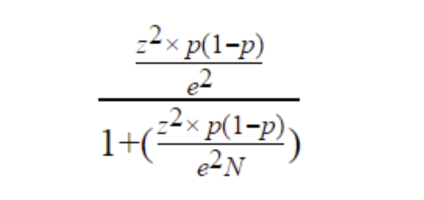
No one wants to work through something like that just to know how many people they should sample. Fortunately, there are several sample size calculators online that simplify knowing how many people to collect data from.

Even if you use a sample size calculator, however, you still need to know some important details about your study. Specifically, you need to know:

• What is the population size in my research?

Population size is the total number of people in the group you are trying to study. If, for example, you were conducting a poll asking U.S. voters about Presidential candidates, then your population of interest would be everyone living in the U.S.—about 330 million people.

Determining the size of the population you’re interested in will often require some background research. For instance, if your company sells digital marketing services and you’re interested in surveying potential customers, it isn’t easy to determine the size of your population. Everyone who is currently engaged in digital marketing may be a potential customer. In situations like these, you can often use industry data or other information to arrive at a reasonable estimate for your population size.

• What margin of error should you use?

Margin of error is a percentage that tells you how much the results from your sample may deviate from the views of the overall population. The smaller your margin of error, the closer your data reflect the opinion of the population at a given confidence level.

Generally speaking, the more people you gather data from the smaller your margin of error. However, because it is almost never feasible to collect data from everyone in the population, some margin of error is necessary in most studies.

• What is your survey’s significance level?

The significance level  is a percentage that tells you how confident you can be that the true population value lies within your margin of error. So, for example, if you are asking people whether they support a candidate for President, the significance level tells you how likely it is that the level of support for the candidate in the population (i.e., people not in your sample) falls within the margin of error found in your sample.

Common significance levels in survey research are 90%, 95%, and 99%.

Once you know the values above, you can plug them into a sample size formula or more conveniently an online calculator to determine your sample size.

The table below displays the necessary sample size for different sized populations and margin of errors. As you can see, even when a population is large, researchers can often understand the entire group with about 1,000 respondents.

• How Many People Should I Invite to My Study?

Sample size calculations tell you how many people you need to complete your survey. What they do not tell you, however, is how many people you need to invite to your survey. To find that number, you need to consider the response rate.

For example, if you are conducting a study of customer satisfaction and you know from previous experience that only about 30% of the people you contact will actually respond to your survey, then you can determine how many people you should invite to the survey to wind up with your desired sample size.

All you have to do is take the number of respondents you need, divide by your expected response rate, and multiple by 100. For example, if you need 500 customers to respond to your survey and you know the response rate is 30%, you should invite about 1,666 people to your study (500/30*100 = 1,666).

Sample size formulas are based on probability sampling techniques—methods that randomly select people from the population to participate in a survey. For most market surveys and academic studies, however, researchers do not use probability sampling methods. Instead they use a mix of convenience and purposive sampling methods that we refer to as controlled sampling .

When surveys and descriptive studies are based on controlled sampling methods, how should researchers calculate sample size?

When the study’s aim is to measure the frequency of something or to describe people’s behavior, we recommend following the calculations made for probability sampling. This often translates to a sample of about 1,000 to 2,000 people. When a study’s aim is to investigate a correlational relationship, however, we recommend sampling between 500 and 1,000 people. More participants in a study will always be better, but these numbers are a useful rule of thumb for researchers seeking to find out how many participants they need to sample.

If you look online, you will find many sources with information for calculating sample size when conducting a survey, but fewer resources for calculating sample size when conducting an experiment. Experiments involve randomly assigning people to different conditions and manipulating variables in order to determine a cause-and-effect relationship. The reason why sample size calculators for experiments are hard to find is simple: experiments are complex and sample size calculations depend on several factors.

The guidance we offer here is to help researchers calculate sample size for some of the simplest and most common experimental designs: t -tests, A/B tests, and chi square tests.

Many businesses today rely on A/B tests. Especially in the digital environment, A/B tests provide an efficient way to learn what kinds of features, messages, and displays cause people to spend more time or money on a website or an app.

For example, one common use of A/B testing is marketing emails. A marketing manager might create two versions of an email, randomly send one to half the company’s customers and randomly send the second to the other half of customers and then measure which email generates more sales.

In many cases , researchers may know they want to conduct an A/B test but be unsure how many people they need in their sample to obtain statistically significant results. In order to begin a sample size calculation, you need to know three things.

1. The significance level .

The significance level represents how sure you want to be that your results are not due to chance. A significance level of .05 is a good starting point, but you may adjust this number up or down depending on the aim of your study.

2. Your desired power.

Statistical tests are only useful when they have enough power to detect an effect if one actually exists. Most researchers aim for 80% power—meaning their tests are sensitive enough to detect an effect 8 out of 10 times if one exists.

3. The minimum effect size you are interested in.

The final piece of information you need is the minimum effect size, or difference between groups, you are interested in. Sometimes there may be a difference between groups, but if the difference is so small that it makes little practical difference to your business, it probably isn’t worth investigating. Determining the minimum effect size you are interested in requires some thought about your goals and the potential impact on your business. 

Once you have decided on the factors above, you can use a sample size calculator to determine how many people you need in each of your study’s conditions.

Let’s say a marketing team wants to test two different email campaigns. They set their significance level at .05 and their power at 80%. In addition, the team determines that the minimum response rate difference between groups that they are interested in is 7.5%. Plugging these numbers into an effect size calculator reveals that the team needs 693 people in each condition of their study, for a total of 1,386.

Sending an email out to 1,386 people who are already on your contact list doesn’t cost too much. But for many other studies, each respondent you recruit will cost money. For this reason, it is important to strongly consider what the minimum effect size of interest is when planning a study.    

When you don’t know what size difference to expect among groups, you can default to one of a few rules of thumb. First, use the effect size of minimum practical significance. By deciding what the minimum difference is between groups that would be meaningful, you can avoid spending resources investigating things that are likely to have little consequences for your business.

A second rule of thumb that is particularly relevant for researchers in academia is to assume an effect size of d = .4. A d = .4 is considered by some to be the smallest effect size that begins to have practical relevance . And fortunately, with this effect size and just two conditions, researchers need about 100 people per condition.

After you know how many people to recruit for your study, the next step is finding your participants. By using CloudResearch’s Prime Panels or MTurk Toolkit, you can gain access to more than 50 million people worldwide in addition to user-friendly tools designed to make running your study easy. We can help you find your sample regardless of what your study entails. Need people from a narrow demographic group? Looking to collect data from thousands of people? Do you need people who are willing to engage in a long or complicated study? Our team has the knowledge and expertise to match you with the right group of participants for your study. Get in touch with us today and learn what we can do for you.

Continue Reading: A Researcher’s Guide to Statistical Significance and Sample Size Calculations

Part 1: What Does It Mean for Research to Be Statistically Significant?

Part 2: How to Calculate Statistical Significance

Related articles, what is data quality and why is it important.

If you were a researcher studying human behavior 30 years ago, your options for identifying participants for your studies were limited. If you worked at a university, you might be...

How to Identify and Handle Invalid Responses to Online Surveys

As a researcher, you are aware that planning studies, designing materials and collecting data each take a lot of work. So when you get your hands on a new dataset,...

SUBSCRIBE TO RECEIVE UPDATES

2024 grant application form, personal and institutional information.

• Full Name * First Last
• Position/Title *
• Affiliated Academic Institution or Research Organization *

Detailed Research Proposal Questions

• Project Title *
• Research Category * - Antisemitism Islamophobia Both
• Objectives *
• Methodology (including who the targeted participants are) *
• Expected Outcomes *
• Significance of the Study *

Budget and Grant Tier Request

• Requested Grant Tier * - $200 $500 $1000 Applicants requesting larger grants may still be eligible for smaller awards if the full amount requested is not granted.
• Budget Justification *

Research Timeline

• Projected Start Date * MM slash DD slash YYYY Preference will be given to projects that can commence soon, preferably before September 2024.
• Estimated Completion Date * MM slash DD slash YYYY Preference will be given to projects that aim to complete within a year.
• Project Timeline *
• Phone This field is for validation purposes and should be left unchanged.

• Name * First Name Last Name
• I would like to request a demo of the Sentry platform
• Comments This field is for validation purposes and should be left unchanged.
• Name * First name Last name
• Email This field is for validation purposes and should be left unchanged.

• Name * First Last
• Name * First and Last
• Please select the best time to discuss your project goals/details to claim your free Sentry pilot for the next 60 days or to receive 10% off your first Managed Research study with Sentry.

• Email * Enter Email Confirm Email
• Organization
• Job Title *

• Skip to main content
• Skip to primary sidebar
• Skip to footer
• QuestionPro

• Solutions Industries Gaming Automotive Sports and events Education Government Travel & Hospitality Financial Services Healthcare Cannabis Technology Use Case NPS+ Communities Audience Contactless surveys Mobile LivePolls Member Experience GDPR Positive People Science 360 Feedback Surveys
• Resources Blog eBooks Survey Templates Case Studies Training Help center

Home Audience

Sample Size Determination: Definition, Formula, and Example

Are you ready to survey your research target? Research surveys help you gain insights from your target audience. The data you collect gives you insights to meet customer needs, leading to increased sales and customer loyalty. Sample size calculation and determination are imperative to the researcher to determine the right number of respondents, keeping in mind the research study’s quality.

So, how should you do the sample size determination? How do you know who should get your survey? How do you decide on the number of the target audience?

Sending out too many surveys can be expensive without giving you a definitive advantage over a smaller sample. But if you send out too few, you won’t have enough data to draw accurate conclusions. 

Knowing how to calculate and determine the appropriate sample size accurately can give you an edge over your competitors. Let’s take a look at what a good sample includes. Also, let’s look at the sample size calculation formula so you can determine the perfect sample size for your next survey.

What is Sample Size?

‘Sample size’ is a market research term used for defining the number of individuals included in conducting research. Researchers choose their sample based on demographics, such as age, gender questions , or physical location. It can be vague or specific. 

For example, you may want to know what people within the 18-25 age range think of your product. Or, you may only require your sample to live in the United States, giving you a wide population range. The total number of individuals in a particular sample is the sample size.

What is sample size determination?

Sample size determination is the process of choosing the right number of observations or people from a larger group to use in a sample. The goal of figuring out the sample size is to ensure that the sample is big enough to give statistically valid results and accurate estimates of population parameters but small enough to be manageable and cost-effective.

In many research studies, getting information from every member of the population of interest is not possible or useful. Instead, researchers choose a sample of people or events that is representative of the whole to study. How accurate and precise the results are can depend a lot on the size of the sample.

Choosing the statistically significant sample size depends on a number of things, such as the size of the population, how precise you want your estimates to be, how confident you want to be in the results, how different the population is likely to be, and how much money and time you have for the study. Statistics are often used to figure out how big a sample should be for a certain type of study and research question.

Figuring out the sample size is important in ensuring that research findings and conclusions are valid and reliable.

Why do you need to determine the sample size?

Let’s say you are a market researcher in the US and want to send out a survey or questionnaire . The survey aims to understand your audience’s feelings toward a new cell phone you are about to launch. You want to know what people in the US think about the new product to predict the phone’s success or failure before launch.

Hypothetically, you choose the population of New York, which is 8.49 million. You use a sample size determination formula to select a sample of 500 individuals that fit into the consumer panel requirement. You can use the responses to help you determine how your audience will react to the new product.

However, determining a sample size requires more than just throwing your survey at as many people as possible. If your estimated sample sizes are too big, it could waste resources, time, and money. A sample size that’s too small doesn’t allow you to gain maximum insights, leading to inconclusive results.

LEARN ABOUT: Survey Sample Sizes

What are the terms used around the sample size?

Before we jump into sample size determination, let’s take a look at the terms you should know:

1. Population size: 

Population size is how many people fit your demographic. For example, you want to get information on doctors residing in North America. Your population size is the total number of doctors in North America. 

Don’t worry! Your population size doesn’t always have to be that big. Smaller population sizes can still give you accurate results as long as you know who you’re trying to represent.

2. Confidence level: 

The confidence level tells you how sure you can be that your data is accurate. It is expressed as a percentage and aligned to the confidence interval. For example, if your confidence level is 90%, your results will most likely be 90% accurate.

3. The margin of error (confidence interval): 

There’s no way to be 100% accurate when it comes to surveys. Confidence intervals tell you how far off from the population means you’re willing to allow your data to fall. 

A margin of error describes how close you can reasonably expect a survey result to fall relative to the real population value. Remember, if you need help with this information, use our margin of error calculator .

4. Standard deviation: 

Standard deviation is the measure of the dispersion of a data set from its mean. It measures the absolute variability of a distribution. The higher the dispersion or variability, the greater the standard deviation and the greater the magnitude of the deviation. 

For example, you have already sent out your survey. How much variance do you expect in your responses? That variation in response is the standard deviation.

Sample size calculation formula – sample size determination

With all the necessary terms defined, it’s time to learn how to determine sample size using a sample calculation formula.

Your confidence level corresponds to a Z-score. This is a constant value needed for this equation. Here are the z-scores for the most common confidence levels:

90% – Z Score = 1.645

95% – Z Score = 1.96

99% – Z Score = 2.576

If you choose a different confidence level, various online tools can help you find your score.

Necessary Sample Size = (Z-score)2 * StdDev*(1-StdDev) / (margin of error)2

Here is an example of how the math works, assuming you chose a 90% confidence level, .6 standard deviation, and a margin of error (confidence interval) of +/- 4%.

((1.64)2 x .6(.6)) / (.04)2

( 2.68x .0.36) / .0016

.9648 / .0016

603 respondents are needed, and that becomes your sample size.

Free Sample Size Calculator

How is a sample size determined?

Determining the right sample size for your survey is one of the most common questions researchers ask when they begin a market research study. Luckily, sample size determination isn’t as hard to calculate as you might remember from an old high school statistics class.

Before calculating your sample size, ensure you have these things in place:

Goals and objectives: 

What do you hope to do with the survey? Are you planning on projecting the results onto a whole demographic or population? Do you want to see what a specific group thinks? Are you trying to make a big decision or just setting a direction? 

Calculating sample size is critical if you’re projecting your survey results on a larger population. You’ll want to make sure that it’s balanced and reflects the community as a whole. The sample size isn’t as critical if you’re trying to get a feel for preferences. 

For example, you’re surveying homeowners across the US on the cost of cooling their homes in the summer. A homeowner in the South probably spends much more money cooling their home in the humid heat than someone in Denver, where the climate is dry and cool. 

For the most accurate results, you’ll need to get responses from people in all US areas and environments. If you only collect responses from one extreme, such as the warm South, your results will be skewed.

Precision level: 

How close do you want the survey results to mimic the true value if everyone responded? Again, if this survey determines how you’re going to spend millions of dollars, then your sample size determination should be exact. 

The more accurate you need to be, the larger the sample you want to have, and the more your sample will have to represent the overall population. If your population is small, say, 200 people, you may want to survey the entire population rather than cut it down with a sample.

Confidence level: 

Think of confidence from the perspective of risk. How much risk are you willing to take on? This is where your Confidence Interval numbers become important. How confident do you want to be — 98% confident, 95% confident? 

Understand that the confidence percentage you choose greatly impacts the number of completions you’ll need for accuracy. This can increase the survey’s length and how many responses you need, which means increased costs for your survey. 

Knowing the actual numbers and amounts behind percentages can help make more sense of your correct sample size needs vs. survey costs. 

For example, you want to be 99% confident. After using the sample size determination formula, you find you need to collect an additional 1000 respondents. 

This, in turn, means you’ll be paying for samples or keeping your survey running for an extra week or two. You have to determine if the increased accuracy is more important than the cost.

Population variability: 

What variability exists in your population? In other words, how similar or different is the population?

If you are surveying consumers on a broad topic, you may have lots of variations. You’ll need a larger sample size to get the most accurate picture of the population. 

However, if you’re surveying a population with similar characteristics, your variability will be less, and you can sample fewer people. More variability equals more samples, and less variability equals fewer samples. If you’re not sure, you can start with 50% variability.

Response rate: 

You want everyone to respond to your survey. Unfortunately, every survey comes with targeted respondents who either never open the study or drop out halfway. Your response rate will depend on your population’s engagement with your product, service organization, or brand. 

The higher the response rate, the higher your population’s engagement level. Your base sample size is the number of responses you must get for a successful survey.

Consider your audience: 

Besides the variability within your population, you need to ensure your sample doesn’t include people who won’t benefit from the results. One of the biggest mistakes you can make in sample size determination is forgetting to consider your actual audience. 

For example, you don’t want to send a survey asking about the quality of local apartment amenities to a group of homeowners.

Select your respondents

Focus on your survey’s objectives: 

You may start with general demographics and characteristics, but can you narrow those characteristics down even more? Narrowing down your audience makes getting a more accurate result from a small sample size easier. 

For example, you want to know how people will react to new automobile technology. Your current population includes anyone who owns a car in a particular market. 

However, you know your target audience is people who drive cars that are less than five years old. You can remove anyone with an older vehicle from your sample because they’re unlikely to purchase your product.

Once you know what you hope to gain from your survey and what variables exist within your population, you can decide how to calculate sample size. Using the formula for determining sample size is a great starting point to get accurate results. 

After calculating the sample size, you’ll want to find reliable customer survey software to help you accurately collect survey responses and turn them into analyzed reports.

LEARN MORE: Population vs Sample

In sample size determination, statistical analysis plan needs careful consideration of the level of significance, effect size, and sample size. 

Researchers must reconcile statistical significance with practical and ethical factors like practicality and cost. A well-designed study with a sufficient sample size can improve the odds of obtaining statistically significant results.

To meet the goal of your survey, you may have to try a few methods to increase the response rate, such as:

• Increase the list of people who receive the survey.
• To reach a wider audience, use multiple distribution channels, such as SMS, website, and email surveys.
• Send reminders to survey participants to complete the survey.
• Offer incentives for completing the survey, such as an entry into a prize drawing or a discount on the respondent’s next order.
• Consider your survey structure and find ways to simplify your questions. The less work someone has to do to complete the survey, the more likely they will finish it. 
• Longer surveys tend to have lower response rates due to the length of time it takes to complete the survey. In this case, you can reduce the number of questions in your survey to increase responses.  

QuestionPro’s sample size calculator makes it easy to find the right sample size for your research based on your desired level of confidence, your margin of error, and the size of the population.

FREE TRIAL         LEARN MORE

Frequently Asked Questions (FAQ)

The four ways to determine sample size are: 1. Power analysis 2. Convenience sampling, 3. Random sampling , 4. Stratified sampling

The three factors that determine sample size are: 1. Effect size, 2. Level of significance 3. Power

Using statistical techniques like power analysis, the minimal detectable effect size, or the sample size formula while taking into account the study’s goals and practical limitations is the best way to calculate the sample size.

The sample size is important because it affects how precise and accurate the results of a study are and how well researchers can spot real effects or relationships between variables.

The sample size is the number of observations or study participants chosen to be representative of a larger group

MORE LIKE THIS

Top 13 A/B Testing Software for Optimizing Your Website

Apr 12, 2024

21 Best Contact Center Experience Software in 2024

Government Customer Experience: Impact on Government Service

Apr 11, 2024

Employee Engagement App: Top 11 For Workforce Improvement 

Apr 10, 2024

Other categories

• Academic Research
• Artificial Intelligence
• Assessments
• Brand Awareness
• Case Studies
• Communities
• Consumer Insights
• Customer effort score
• Customer Engagement
• Customer Experience
• Customer Loyalty
• Customer Research
• Customer Satisfaction
• Employee Benefits
• Employee Engagement
• Employee Retention
• Friday Five
• General Data Protection Regulation
• Insights Hub
• Life@QuestionPro
• Market Research
• Mobile diaries
• Mobile Surveys
• New Features
• Online Communities
• Question Types
• Questionnaire
• QuestionPro Products
• Release Notes
• Research Tools and Apps
• Revenue at Risk
• Survey Templates
• Training Tips
• Uncategorized
• Video Learning Series
• What’s Coming Up
• Workforce Intelligence

• Dissertations
• Qualitative Research
• Quantitative Research
• Academic Writing
• Getting Published

News & Events

How to determine the sample size for your study.

• May 1, 2017
• Posted by: Mike Rucker
• Category: Research

When conducting quantitative research, it is very important to determine the sample size for your study. Your sample needs to represent the target population you plan to examine. Sample size calculation should be done before you set off to collect any of your data. Almost all researchers generally like to work with large samples. However, this is not always feasible — especially for students (time, money, resources, etc.) — so it is a good idea to assess your need before any real research takes place to determine how many participants you really need (and can feasibly get) before planning your research.

This post presents a brief overview of sample size calculations and covers some of the basics. For complex cases and more detail, you will probably require more thorough text on the subject (see: Sample Size Determination and Power ).

A Few Terms That Relate to the Size of Your Sample

Here are some expressions you will most likely come across when designing your study and deciding on a sample size.

• Population – This is the complete set of data points, for example, all Americans.
• Target population – This is the complete group for which you are studying; your data will have specific characteristics (demographics, clinical characteristics) that you are interested in — for example, Americans over the age of 65, who live at home and have had a stroke in the past 6 months.
• Sample – A subset of the target population that represents the target population.
• Margin of Error – The margin of error is about a degree of uncertainty in statistics. How much error will you allow? We would like the mean of our data to represent the mean of the target population; however, this is generally not going to happen. The margin of error tells us how much higher or lower than the true value will we let our sample mean fall. In articles, you usually see a +/-5% or +/-3% margin of error.
• Confidence Interval – Confidence interval (CI) is usually set at 90%, 95% or 99%. It tells us how confident we are that if the study was repeated again and again, we would get the same results. If confidence level is 95%, we would get the same results in 95% of the cases.
• Standard Deviation – Standard deviation tells us the variation in the data from your sample.
• Power – This refers to the chance of missing a real difference (‘false negatives’). Usually, studies have a power of around 80%, which means that you accept the possibility that in 20% of the cases, the real difference was missed (you concluded there was no effect when there was one). Larger samples generally yield higher statistical power.

How to Calculate a Sample Size

It is fairly easy to determine your desired sample size. Formulas found in textbooks often appear very intimidating. However, they can be broken down and simplified if you are familiar with the above terms.

Scott Smith , Ph.D., presents a rather simpler version.  His formula for size calculation goes as follows:

(Z value) 2 X standard deviation (1-standard deviation)/(margin of error) 2 = n

This formula, however, can only be used for large populations or unknown population sizes.

The Z-value or Z-score corresponds with your chosen confidence level.  There are usually Z tables available that tell you the Z-score. You can then insert that value into the formula. Below are values for the most commonly used confidence intervals.

You can use the formula to calculate a sample size for a confidence level of 99% and margin of error +/-1% (.01), using the standard deviation suggestion of .05.

(2.58) 2 *0.5(1-0.5)/(0.01) 2 = 6.656*0.5(0.5)/0.0001= 16,641

The sample size for the chosen parameters should be 16,641, which is a very large sample. To make it a more realistic number, you might consider reducing your confidence level and margin of error. If you reduce it to 95% confidence level and 5% margin of error, you get a more manageable 384.16 participants, which you round up to 385.

Software for Calculating Your Sample Size

If this still appears like a pretty cumbersome task (or you have a smaller population size), you can also turn to various software programs and websites that will calculate the size for you. An example of such a site is The Survey System , which offers a free online sample size calculator. Another option is Survey Monkey ’s sample size calculator, which can also be accessed online. These calculators usually ask you to enter your target population size, confidence level and margin of error.

You can also ask for guidance and assistance from other members of your department who might be more skilled at statistics. For additional ideas on how to get help with statistics, you can have a look at this post .

Root out friction in every digital experience, super-charge conversion rates, and optimize digital self-service

Uncover insights from any interaction, deliver AI-powered agent coaching, and reduce cost to serve

Increase revenue and loyalty with real-time insights and recommendations delivered to teams on the ground

Know how your people feel and empower managers to improve employee engagement, productivity, and retention

Take action in the moments that matter most along the employee journey and drive bottom line growth

Whatever they’re are saying, wherever they’re saying it, know exactly what’s going on with your people

Get faster, richer insights with qual and quant tools that make powerful market research available to everyone

Run concept tests, pricing studies, prototyping + more with fast, powerful studies designed by UX research experts

Track your brand performance 24/7 and act quickly to respond to opportunities and challenges in your market

Explore the platform powering Experience Management

• Free Account
• For Digital
• For Customer Care
• For Human Resources
• For Researchers
• Financial Services
• All Industries

Popular Use Cases

• Customer Experience
• Employee Experience
• Employee Exit Interviews
• Net Promoter Score
• Voice of Customer
• Customer Success Hub
• Product Documentation
• Training & Certification
• XM Institute
• Popular Resources
• Customer Stories
• Market Research
• Artificial Intelligence
• Partnerships
• Marketplace

The annual gathering of the experience leaders at the world’s iconic brands building breakthrough business results, live in Salt Lake City.

• English/AU & NZ
• Español/Europa
• Español/América Latina
• Português Brasileiro
• REQUEST DEMO
• Experience Management
• How To Determine Sample Size

Try Qualtrics for free

How to determine sample size.

12 min read Sample size can make or break your research project. Here’s how to master the delicate art of choosing the right sample size.

Author:  Will Webster

Sample size is the beating heart of any research project. It’s the invisible force that gives life to your data, making your findings robust, reliable and believable.

Sample size is what determines if you see a broad view or a focus on minute details; the art and science of correctly determining it involves a careful balancing act. Finding an appropriate sample size demands a clear understanding of the level of detail you wish to see in your data and the constraints you might encounter along the way.

Remember, whether you’re studying a small group or an entire population, your findings are only ever as good as the sample you choose.

Free eBook: Empower your market research efforts today

Let’s delve into the world of sampling and uncover the best practices for determining sample size for your research.

“How much sample do we need?” is one of the most commonly-asked questions and stumbling points in the early stages of research design . Finding the right answer to it requires first understanding and answering two other questions:

How important is statistical significance to you and your stakeholders?

What are your real-world constraints.

At the heart of this question is the goal to confidently differentiate between groups, by describing meaningful differences as statistically significant. Statistical significance isn’t a difficult concept, but it needs to be considered within the unique context of your research and your measures.

First, you should consider when you deem a difference to be meaningful in your area of research. While the standards for statistical significance are universal, the standards for “meaningful difference” are highly contextual.

For example, a 10% difference between groups might not be enough to merit a change in a marketing campaign for a breakfast cereal, but a 10% difference in efficacy of breast cancer treatments might quite literally be the difference between life and death for hundreds of patients. The exact same magnitude of difference has very little meaning in one context, but has extraordinary meaning in another. You ultimately need to determine the level of precision that will help you make your decision.

Within sampling, the lowest amount of magnification – or smallest sample size – could make the most sense, given the level of precision needed, as well as timeline and budgetary constraints.

If you’re able to detect statistical significance at a difference of 10%, and 10% is a meaningful difference, there is no need for a larger sample size, or higher magnification. However, if the study will only be useful if a significant difference is detected for smaller differences – say, a difference of 5% — the sample size must be larger to accommodate this needed precision. Similarly, if 5% is enough, and 3% is unnecessary, there is no need for a larger statistically significant sample size.

You should also consider how much you expect your responses to vary. When there isn’t a lot of variability in response, it takes a lot more sample to be confident that there are statistically significant differences between groups.

For instance, it will take a lot more sample to find statistically significant differences between groups if you are asking, “What month do you think Christmas is in?” than if you are asking, “How many miles are there between the Earth and the moon?”. In the former, nearly everybody is going to give the exact same answer, while the latter will give a lot of variation in responses. Simply put, when your variables do not have a lot of variance, larger sample sizes make sense.

Statistical significance

The likelihood that the results of a study or experiment did not occur randomly or by chance, but are meaningful and indicate a genuine effect or relationship between variables.

Magnitude of difference

The size or extent of the difference between two or more groups or variables, providing a measure of the effect size or practical significance of the results.

Actionable insights

Valuable findings or conclusions drawn from data analysis that can be directly applied or implemented in decision-making processes or strategies to achieve a particular goal or outcome.

It’s crucial to understand the differences between the concepts of “statistical significance”, “magnitude of difference” and “actionable insights” – and how they can influence each other:

• Even if there is a statistically significant difference, it doesn’t mean the magnitude of the difference is large: with a large enough sample, a 3% difference could be statistically significant
• Even if the magnitude of the difference is large, it doesn’t guarantee that this difference is statistically significant: with a small enough sample, an 18% difference might not be statistically significant
• Even if there is a large, statistically significant difference, it doesn’t mean there is a story, or that there are actionable insights

There is no way to guarantee statistically significant differences at the outset of a study – and that is a good thing.

Even with a sample size of a million, there simply may not be any differences – at least, any that could be described as statistically significant. And there are times when a lack of significance is positive.

Imagine if your main competitor ran a multi-million dollar ad campaign in a major city and a huge pre-post study to detect campaign effects, only to discover that there were no statistically significant differences in brand awareness . This may be terrible news for your competitor, but it would be great news for you.

With Stats iQ™ you can analyze your research results and conduct significance testing

As you determine your sample size, you should consider the real-world constraints to your research.

Factors revolving around timings, budget and target population are among the most common constraints, impacting virtually every study. But by understanding and acknowledging them, you can definitely navigate the practical constraints of your research when pulling together your sample.

Timeline constraints

Gathering a larger sample size naturally requires more time. This is particularly true for elusive audiences, those hard-to-reach groups that require special effort to engage. Your timeline could become an obstacle if it is particularly tight, causing you to rethink your sample size to meet your deadline.

Budgetary constraints

Every sample, whether large or small, inexpensive or costly, signifies a portion of your budget. Samples could be like an open market; some are inexpensive, others are pricey, but all have a price tag attached to them.

Population constraints

Sometimes the individuals or groups you’re interested in are difficult to reach; other times, they’re a part of an extremely small population. These factors can limit your sample size even further.

What’s a good sample size?

A good sample size really depends on the context and goals of the research. In general, a good sample size is one that accurately represents the population and allows for reliable statistical analysis.

Larger sample sizes are typically better because they reduce the likelihood of sampling errors and provide a more accurate representation of the population. However, larger sample sizes often increase the impact of practical considerations, like time, budget and the availability of your audience. Ultimately, you should be aiming for a sample size that provides a balance between statistical validity and practical feasibility.

4 tips for choosing the right sample size

Choosing the right sample size is an intricate balancing act, but following these four tips can take away a lot of the complexity.

1) Start with your goal

The foundation of your research is a clearly defined goal. You need to determine what you’re trying to understand or discover, and use your goal to guide your research methods – including your sample size.

If your aim is to get a broad overview of a topic, a larger, more diverse sample may be appropriate. However, if your goal is to explore a niche aspect of your subject, a smaller, more targeted sample might serve you better. You should always align your sample size with the objectives of your research.

2) Know that you can’t predict everything

Research is a journey into the unknown. While you may have hypotheses and predictions, it’s important to remember that you can’t foresee every outcome – and this uncertainty should be considered when choosing your sample size.

A larger sample size can help to mitigate some of the risks of unpredictability, providing a more diverse range of data and potentially more accurate results. However, you shouldn’t let the fear of the unknown push you into choosing an impractically large sample size.

3) Plan for a sample that meets your needs and considers your real-life constraints

Every research project operates within certain boundaries – commonly budget, timeline and the nature of the sample itself. When deciding on your sample size, these factors need to be taken into consideration.

Be realistic about what you can achieve with your available resources and time, and always tailor your sample size to fit your constraints – not the other way around.

4) Use best practice guidelines to calculate sample size

There are many established guidelines and formulas that can help you in determining the right sample size.

The easiest way to define your sample size is using a sample size calculator , or you can use a manual sample size calculation if you want to test your math skills. Cochran’s formula is perhaps the most well known equation for calculating sample size, and widely used when the population is large or unknown.

Beyond the formula, it’s vital to consider the confidence interval, which plays a significant role in determining the appropriate sample size – especially when working with a random sample – and the sample proportion. This represents the expected ratio of the target population that has the characteristic or response you’re interested in, and therefore has a big impact on your correct sample size.

If your population is small, or its variance is unknown, there are steps you can still take to determine the right sample size. Common approaches here include conducting a small pilot study to gain initial estimates of the population variance, and taking a conservative approach by assuming a larger variance to ensure a more representative sample size.

Empower your market research

Conducting meaningful research and extracting actionable intelligence are priceless skills in today’s ultra competitive business landscape. It’s never been more crucial to stay ahead of the curve by leveraging the power of market research to identify opportunities, mitigate risks and make informed decisions.

Equip yourself with the tools for success with our essential eBook, “The ultimate guide to conducting market research” .

With this front-to-back guide, you’ll discover the latest strategies and best practices that are defining effective market research. Learn about practical insights and real-world applications that are demonstrating the value of research in driving business growth and innovation.

Related resources

Selection bias 11 min read, systematic random sampling 15 min read, convenience sampling 18 min read, probability sampling 8 min read, non-probability sampling 17 min read, stratified random sampling 12 min read, simple random sampling 9 min read, request demo.

Ready to learn more about Qualtrics?

An official website of the United States government

The .gov means it’s official. Federal government websites often end in .gov or .mil. Before sharing sensitive information, make sure you’re on a federal government site.

The site is secure. The https:// ensures that you are connecting to the official website and that any information you provide is encrypted and transmitted securely.

• Publications
• Account settings

Preview improvements coming to the PMC website in October 2024. Learn More or Try it out now .

• Advanced Search
• Journal List
• Indian J Psychol Med
• v.42(1); Jan-Feb 2020

Sample Size and its Importance in Research

Chittaranjan andrade.

Clinical Psychopharmacology Unit, Department of Clinical Psychopharmacology and Neurotoxicology, National Institute of Mental Health and Neurosciences, Bengaluru, Karnataka, India

The sample size for a study needs to be estimated at the time the study is proposed; too large a sample is unnecessary and unethical, and too small a sample is unscientific and also unethical. The necessary sample size can be calculated, using statistical software, based on certain assumptions. If no assumptions can be made, then an arbitrary sample size is set for a pilot study. This article discusses sample size and how it relates to matters such as ethics, statistical power, the primary and secondary hypotheses in a study, and findings from larger vs. smaller samples.

Studies are conducted on samples because it is usually impossible to study the entire population. Conclusions drawn from samples are intended to be generalized to the population, and sometimes to the future as well. The sample must therefore be representative of the population. This is best ensured by the use of proper methods of sampling. The sample must also be adequate in size – in fact, no more and no less.

SAMPLE SIZE AND ETHICS

A sample that is larger than necessary will be better representative of the population and will hence provide more accurate results. However, beyond a certain point, the increase in accuracy will be small and hence not worth the effort and expense involved in recruiting the extra patients. Furthermore, an overly large sample would inconvenience more patients than might be necessary for the study objectives; this is unethical. In contrast, a sample that is smaller than necessary would have insufficient statistical power to answer the primary research question, and a statistically nonsignificant result could merely be because of inadequate sample size (Type 2 or false negative error). Thus, a small sample could result in the patients in the study being inconvenienced with no benefit to future patients or to science. This is also unethical.

In this regard, inconvenience to patients refers to the time that they spend in clinical assessments and to the psychological and physical discomfort that they experience in assessments such as interviews, blood sampling, and other procedures.

ESTIMATING SAMPLE SIZE

So how large should a sample be? In hypothesis testing studies, this is mathematically calculated, conventionally, as the sample size necessary to be 80% certain of identifying a statistically significant outcome should the hypothesis be true for the population, with P for statistical significance set at 0.05. Some investigators power their studies for 90% instead of 80%, and some set the threshold for significance at 0.01 rather than 0.05. Both choices are uncommon because the necessary sample size becomes large, and the study becomes more expensive and more difficult to conduct. Many investigators increase the sample size by 10%, or by whatever proportion they can justify, to compensate for expected dropout, incomplete records, biological specimens that do not meet laboratory requirements for testing, and other study-related problems.

Sample size calculations require assumptions about expected means and standard deviations, or event risks, in different groups; or, upon expected effect sizes. For example, a study may be powered to detect an effect size of 0.5; or a response rate of 60% with drug vs. 40% with placebo.[ 1 ] When no guesstimates or expectations are possible, pilot studies are conducted on a sample that is arbitrary in size but what might be considered reasonable for the field.

The sample size may need to be larger in multicenter studies because of statistical noise (due to variations in patient characteristics, nonspecific treatment characteristics, rating practices, environments, etc. between study centers).[ 2 ] Sample size calculations can be performed manually or using statistical software; online calculators that provide free service can easily be identified by search engines. G*Power is an example of a free, downloadable program for sample size estimation. The manual and tutorial for G*Power can also be downloaded.

PRIMARY AND SECONDARY ANALYSES

The sample size is calculated for the primary hypothesis of the study. What is the difference between the primary hypothesis, primary outcome and primary outcome measure? As an example, the primary outcome may be a reduction in the severity of depression, the primary outcome measure may be the Montgomery-Asberg Depression Rating Scale (MADRS) and the primary hypothesis may be that reduction in MADRS scores is greater with the drug than with placebo. The primary hypothesis is tested in the primary analysis.

Studies almost always have many hypotheses; for example, that the study drug will outperform placebo on measures of depression, suicidality, anxiety, disability and quality of life. The sample size necessary for adequate statistical power to test each of these hypotheses will be different. Because a study can have only one sample size, it can be powered for only one outcome, the primary outcome. Therefore, the study would be either overpowered or underpowered for the other outcomes. These outcomes are therefore called secondary outcomes, and are associated with secondary hypotheses, and are tested in secondary analyses. Secondary analyses are generally considered exploratory because when many hypotheses in a study are each tested at a P < 0.05 level for significance, some may emerge statistically significant by chance (Type 1 or false positive errors).[ 3 ]

INTERPRETING RESULTS

Here is an interesting question. A test of the primary hypothesis yielded a P value of 0.07. Might we conclude that our sample was underpowered for the study and that, had our sample been larger, we would have identified a significant result? No! The reason is that larger samples will more accurately represent the population value, whereas smaller samples could be off the mark in either direction – towards or away from the population value. In this context, readers should also note that no matter how small the P value for an estimate is, the population value of that estimate remains the same.[ 4 ]

On a parting note, it is unlikely that population values will be null. That is, for example, that the response rate to the drug will be exactly the same as that to placebo, or that the correlation between height and age at onset of schizophrenia will be zero. If the sample size is large enough, even such small differences between groups, or trivial correlations, would be detected as being statistically significant. This does not mean that the findings are clinically significant.

Financial support and sponsorship

Conflicts of interest.

There are no conflicts of interest.