hypothesis test simple linear regression

• school Campus Bookshelves
• menu_book Bookshelves
• perm_media Learning Objects
• login Login
• how_to_reg Request Instructor Account
• hub Instructor Commons
• Download Page (PDF)
• Download Full Book (PDF)
• Periodic Table
• Physics Constants
• Scientific Calculator
• Reference & Cite
• Tools expand_more
• Readability

selected template will load here

This action is not available.

12.2.1: Hypothesis Test for Linear Regression

• Last updated
• Save as PDF
• Page ID 34850

• Rachel Webb
• Portland State University

To test to see if the slope is significant we will be doing a two-tailed test with hypotheses. The population least squares regression line would be \(y = \beta_{0} + \beta_{1} + \varepsilon\) where \(\beta_{0}\) (pronounced “beta-naught”) is the population \(y\)-intercept, \(\beta_{1}\) (pronounced “beta-one”) is the population slope and \(\varepsilon\) is called the error term.

If the slope were horizontal (equal to zero), the regression line would give the same \(y\)-value for every input of \(x\) and would be of no use. If there is a statistically significant linear relationship then the slope needs to be different from zero. We will only do the two-tailed test, but the same rules for hypothesis testing apply for a one-tailed test.

We will only be using the two-tailed test for a population slope.

The hypotheses are:

\(H_{0}: \beta_{1} = 0\) \(H_{1}: \beta_{1} \neq 0\)

The null hypothesis of a two-tailed test states that there is not a linear relationship between \(x\) and \(y\). The alternative hypothesis of a two-tailed test states that there is a significant linear relationship between \(x\) and \(y\).

Either a t-test or an F-test may be used to see if the slope is significantly different from zero. The population of the variable \(y\) must be normally distributed.

F-Test for Regression

An F-test can be used instead of a t-test. Both tests will yield the same results, so it is a matter of preference and what technology is available. Figure 12-12 is a template for a regression ANOVA table,

where \(n\) is the number of pairs in the sample and \(p\) is the number of predictor (independent) variables; for now this is just \(p = 1\). Use the F-distribution with degrees of freedom for regression = \(df_{R} = p\), and degrees of freedom for error = \(df_{E} = n - p - 1\). This F-test is always a right-tailed test since ANOVA is testing the variation in the regression model is larger than the variation in the error.

Use an F-test to see if there is a significant relationship between hours studied and grade on the exam. Use \(\alpha\) = 0.05.

T-Test for Regression

If the regression equation has a slope of zero, then every \(x\) value will give the same \(y\) value and the regression equation would be useless for prediction. We should perform a t-test to see if the slope is significantly different from zero before using the regression equation for prediction. The numeric value of t will be the same as the t-test for a correlation. The two test statistic formulas are algebraically equal; however, the formulas are different and we use a different parameter in the hypotheses.

The formula for the t-test statistic is \(t = \frac{b_{1}}{\sqrt{ \left(\frac{MSE}{SS_{xx}}\right) }}\)

Use the t-distribution with degrees of freedom equal to \(n - p - 1\).

The t-test for slope has the same hypotheses as the F-test:

Use a t-test to see if there is a significant relationship between hours studied and grade on the exam, use \(\alpha\) = 0.05.

If you could change one thing about college, what would it be?

Graduate faster

Better quality online classes

Flexible schedule

Access to top-rated instructors

The Complete Guide To Simple Regression Analysis

08.08.2023 • 8 min read

Sarah Thomas

Subject Matter Expert

Learn what simple regression analysis means and why it’s useful for analyzing data, and how to interpret the results.

In This Article

What Is Simple Linear Regression Analysis?

Linear regression equation, how to perform linear regression, linear regression assumptions, how do you find the regression line, how to interpret the results of simple regression.

What is the relationship between parental income and educational attainment or hours spent on social media and anxiety levels? Regression is a versatile statistical tool that can help you answer these types of questions. It’s a tool that lets you model the relationship between two or more variables .

The applications of regression are endless. You can use it as a machine learning algorithm to make predictions. You can use it to establish correlations, and in some cases, you can use it to uncover causal links in your data.

In this article, we’ll tell you everything you need to know about the most basic form of regression analysis: the simple linear regression model.

Simple linear regression is a statistical tool you can use to evaluate correlations between a single independent variable (X) and a single dependent variable (Y). The model fits a straight line to data collected for each variable, and using this line, you can estimate the correlation between X and Y and predict values of Y using values of X.

As a quick example, imagine you want to explore the relationship between weight (X) and height (Y). You collect data from ten randomly selected individuals, and you plot your data on a scatterplot like the one below.

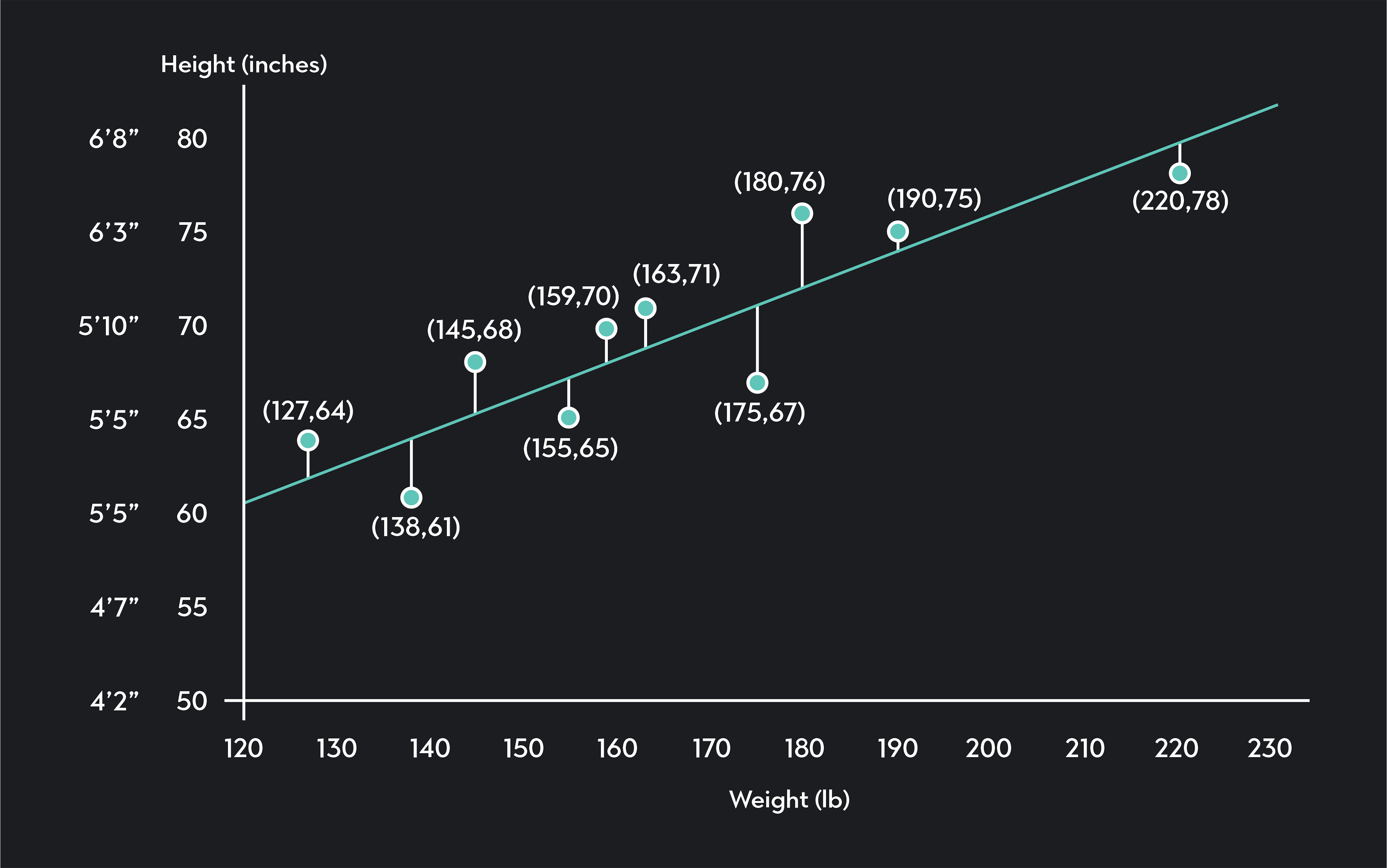
In the scatterplot, each point represents data collected for one of the individuals in your sample. The blue line is your regression line. It models the relationship between weight and height using observed data. Not surprisingly, we see ‌the regression line is upward-sloping, indicating a positive correlation between weight and height. Taller people tend to be heavier than shorter people.

Once you have this line, you can measure how strong the correlation is between height and weight. You can estimate the height of somebody ‌not in your sample by plugging their weight into the regression equation.

The equation for a simple linear regression is:

X is your independent variable

Y is an estimate of your dependent variable

β 0 \beta_0 β 0 ​ is the constant or intercept of the regression line, which is the value of Y when X is equal to zero

β 1 \beta_1 β 1 ​ is the regression coefficient, which is the slope of the regression line and your estimate for the change in Y given a 1-unit change in X

ε \varepsilon ε is the error term of the regression

You may notic‌e the formula for a regression looks very similar to the equation of a line (y=mX+b). That’s because linear regression is a line! It’s a line fitted to data that you can use to estimate the values of one variable using the value of a correlated variable.

You can build a simple linear regression model in 5 steps.

1. Collect data

Collect data for two variables (X and Y). Y is your dependent variable, which is the variable you want to estimate using the regression. X is your independent variable—the variable you use as an input in your regression.

2. Plot the data on a scatter plot

Plot the values of X and Y on a scatter plot with values of X plotted along the horizontal x-axis and values of Y plotted on the vertical y-axis.

3. Calculate a correlation coefficient

Calculate a correlation coefficient to determine the strength of the linear relationship between your two variables.

4. Fit a regression to the data

Find the regression line using the ordinary least-squares method. (You can do this by hand; but it’s much easier to use statistical software like Desmos, Excel, R, or Stata.)

5. Assess the regression line

Once you have the regression line, assess how well your model performs by checking to see how well the model predicts values of Y.

The key assumptions we make when using a simple linear regression model are:

The relationship between X and Y (if it exists) is linear.

Independence

The residuals of your model are independent.

Homoscedasticity

The variance of the residual is constant across values of the independent variable.

The residuals are normally distributed .

You should not use a simple linear regression unless it’s reasonable to make these assumptions.

Simple linear regression involves fitting a straight line to your dataset. We call this line the line of best fit or the regression line. The most common method for finding this line is OLS (or the Ordinary Least Squares Method).

In OLS, we find the regression line by minimizing the sum of squared residuals —also called squared errors. Anytime you draw a straight line through your data, there will be a vertical distance between each ‌point on your scatter plot and the regression line. These vertical distances are called residuals (or errors).

They represent the difference between the actual values of your dependent variable Y i Y_i Y i ​ , and the predicted value of that variable, Y ^ i \widehat{Y}_i Y i ​ . The regression you find with OLS is the line that minimizes the sum of squared residuals.

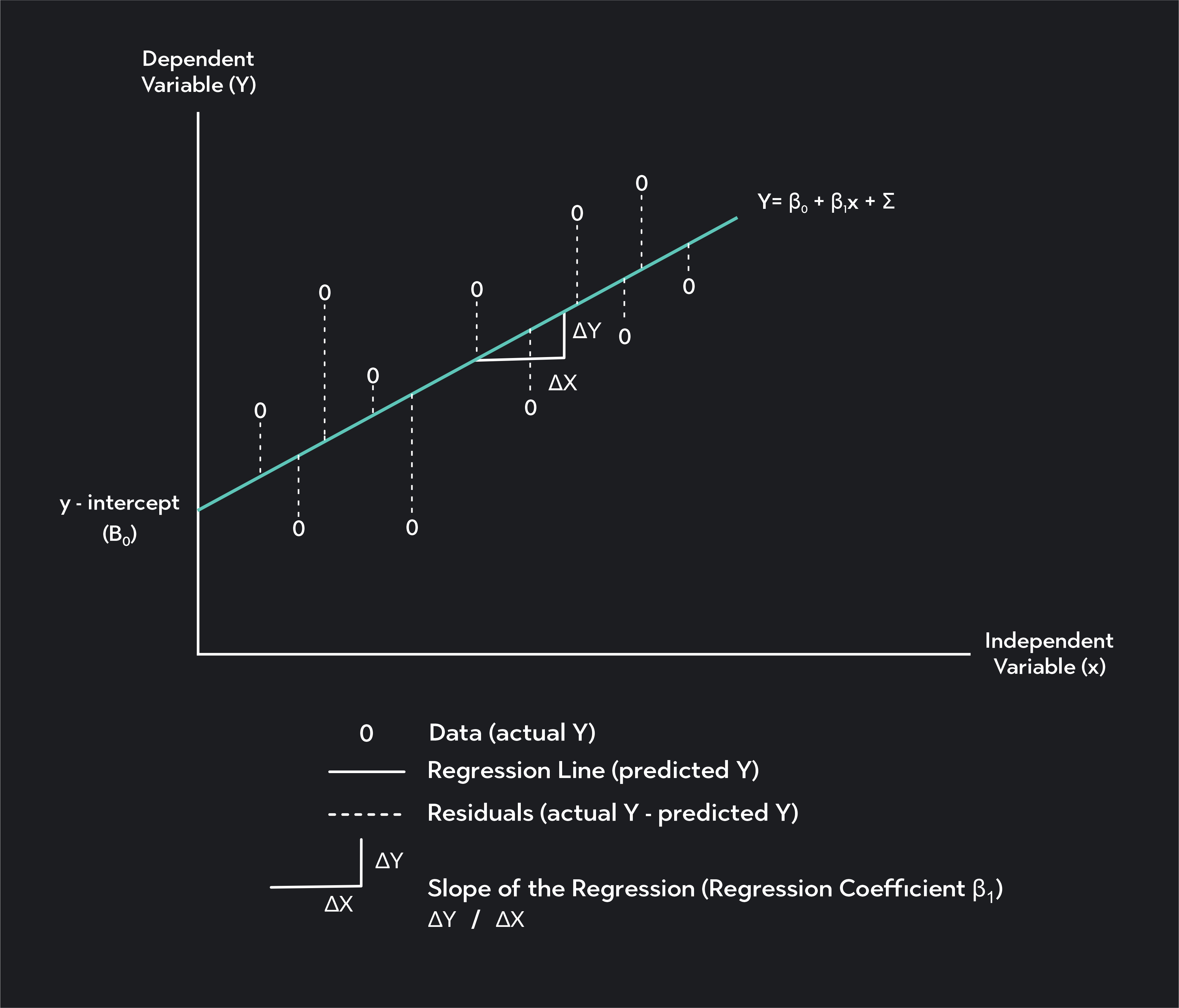
You can calculate the OLS regression line by hand, but it’s much easier to do so using statistical software like Excel, Desmos, R, or Stata. In this video, Professor AnnMaria De Mars explains how to find the OLS regression equation using Desmos.

Depending on the software you use, the results of your regression analysis may look ‌different. In general, however, your software will display output tables summarizing the main characteristics of your regression.

The values you should be looking for in these output tables fall under three categories:

Coefficients

Regression statistics

This is the β 0 \beta_0 β 0 ​ value in your regression equation. It is the y-intercept of your regression line, and it is the estimate of Y when X is equal to zero.

Next to your intercept, you’ll see columns in the table showing additional information about the intercept. These include a standard error, p-value, T-stat, and confidence interval. You can use these values to test whether the estimate of your intercept is statistically significant .

Regression coefficient

This is the β 1 \beta_1 β 1 ​ of your regression equation. It’s the slope of the regression line, and it tells you how much Y should change in response to a 1-unit change in X.

Similar to the intercept, the regression coefficient will have columns to the right of it. They'll show a standard error, p-value , T-stat, and confidence interval. Use these values to test whether your parameter estimate of β 1 \beta_1 β 1 ​ is statistically significant.

Regression Statistics

Correlation coefficient (or multiple r).

This is the Pearson Correlation coefficient. It measures the strength of the correlation between X and Y.

R-squared (or the coefficient of determination)

We calculate this value by squaring the correlation coefficient. The independent variable can explain how much of the variance in your dependent variable. You can convert R 2 R^2 R 2 into a percentage by multiplying it by 100.

Standard error of the residuals

The standard error of the residuals is the average value of the errors in your model. It is the average vertical distance between each point on your scatter plot and the regression line. We measure this value in the same units as your dependent variable.

Degrees of freedom

In simple linear regression, the degrees of freedom equal the number of data points you used minus the two estimated parameters. The parameters are the intercept and regression coefficient.

Some software will also output a 5-number summary of your residuals. It'll show the minimum, first quartile , median , third quartile, and maximum values of your residuals.

P-value (or Significance F) - This is the p-value of your regression model.

It returns a hypothesis test's results where the null hypothesis is that no relationship exists between X and Y. The alternative hypothesis is that a linear relationship exists between X and Y.

If you are using a significance level (or alpha level) of 0.05, you would reject the null hypothesis if the p-value is less than or equal to 0.05. You would fail to reject the null hypothesis if your p-value is greater than 0.05.

What are correlations?

A correlation is a measure of the relationship between two variables.

Positive Correlations - If two variables, X and Y, have a positive linear correlation, Y tends to increase as X increases, and Y tends to decrease as X decreases. In other words, the two variables tend to move together in the same direction.

Negative Correlations - Two variables, X and Y, have a negative correlation if Y tends to increase as X decreases and Y tends to decrease as X increases. (i.e., The values of the two variables tend to move in opposite directions).

What’s the difference between the dependent and independent variables in a regression?

A simple linear regression involves two variables: X, the input or independent variable, and Y, the output or dependent variable. The independent variable is the variable you want to estimate using the regression. Its estimated value “depends” on the parameters and other variables of the model.

The independent variable—also called the predictor variable—is an input in the model. Its value does not depend on the other elements of the model.

Is the correlation coefficient the same as the regression coefficient?

The correlation coefficient and the regression coefficient will both have the same sign (positive or negative), but they are not the same. The only case where these two values will be equal is when the values of X and Y have been standardized to the same scale.

What is a correlation coefficient?

A correlation coefficient—or Pearson’s correlation coefficient —measures the strength of the linear relationship between X and Y. It’s a number ranging between -1 and 1. The closer a coefficient correlation is to 0, the weaker the correlation is between X and Y.

The closer the correlation coefficient is to 1 or -1, the stronger the correlation. Points on a scatter plot will be more dispersed around the regression line when the correlation between X and Y is weak, and the points will be more tightly clustered around the regression line when the correlation is strong.

What is the regression coefficient?

The regression coefficient, β 1 \beta_1 β 1 ​ , is the slope of the regression line. It provides you with an estimate of how much the dependent variable, Y, will change in response to a 1-unit increase in the dependent variable, X.

The regression coefficient can be any number from − ∞ -\infty − ∞ to ∞ \infty ∞ . A positive regression coefficient implies a positive correlation between X and Y, and a negative regression coefficient implies a negative correlation.

Can I use linear regression in Excel?

Yes. The easiest way to add a simple linear regression line in Excel is to install and use Excel’s “Analysis Toolpak” add-in. To do this, go to Tools > Excel Add-ins and select the “Analysis Toolpak.”

Next, follow these steps.

In your spreadsheet, enter your data for X and Y in two columns

Navigate to the “Data” tab and click on the “Data Analysis” icon

From the list of analysis tools, select “Regression” and click “OK”

Select the data for Y and X respectively where it says “Input Y Range” and “Input X Range”

If you’ve labeled your columns with the names of your X and Y variables, click on the “Labels” checkbox.

You can further customize where you want your regression in your workbook and what additional information you would like Excel to display.

Once you’ve finished customizing, click “OK”

Your regression results will display next to your data or in a new sheet.

Is linear regression used to establish causal relationships?

Correlations are not equivalent to causation. If two variables are correlated, you cannot immediately conclude ‌one causes the other to change. A linear regression will immediately indicate whether two variables correlate. But you’ll need to include more variables in your model and use regression with causal theories to draw conclusions about causal relationships.

What are some other types of regression analysis?

Simple linear regression is the most basic form of regression analysis. It involves ‌one independent variable and one dependent variable. Once you get a handle on this model, you can move on to more sophisticated forms of regression analysis. These include multiple linear regression and nonlinear regression.

Multiple linear regression is a model that estimates the linear relationship between variables using one dependent variable and multiple predictor variables. Nonlinear regression is a method used to estimate nonlinear relationships between variables.

Explore Outlier's Award-Winning For-Credit Courses

Outlier (from the co-founder of MasterClass) has brought together some of the world's best instructors, game designers, and filmmakers to create the future of online college.

Check out these related courses:

Intro to Statistics

How data describes our world.

Intro to Microeconomics

Why small choices have big impact.

Intro to Macroeconomics

How money moves our world.

Intro to Psychology

The science of the mind.

Related Articles

Calculating Logarithmic Regression Step-By-Step

Learn about logarithmic regression and the steps to calculate it. We’ll also break down what a logarithmic function is, why it’s useful, and a few examples.

What Is the Interquartile Range (IQR)?

Learn what the interquartile range is, why it’s used in Statistics and how to calculate it. Also read about how it can be helpful for finding outliers.

Calculate Outlier Formula: A Step-By-Step Guide

This article is an overview of the outlier formula and how to calculate it step by step. It’s also packed with examples and FAQs to help you understand it.

Further Reading

What is statistical significance & why learn it, mean absolute deviation (mad) - meaning & formula, discrete & continuous variables with examples, population vs. sample: the big difference, why is statistics important, how to make a box plot.

Linear regression - Hypothesis testing

by Marco Taboga , PhD

This lecture discusses how to perform tests of hypotheses about the coefficients of a linear regression model estimated by ordinary least squares (OLS).

Table of contents

Normal vs non-normal model

The linear regression model, matrix notation, tests of hypothesis in the normal linear regression model, test of a restriction on a single coefficient (t test), test of a set of linear restrictions (f test), tests based on maximum likelihood procedures (wald, lagrange multiplier, likelihood ratio), tests of hypothesis when the ols estimator is asymptotically normal, test of a restriction on a single coefficient (z test), test of a set of linear restrictions (chi-square test), learn more about regression analysis.

The lecture is divided in two parts:

in the first part, we discuss hypothesis testing in the normal linear regression model , in which the OLS estimator of the coefficients has a normal distribution conditional on the matrix of regressors;

in the second part, we show how to carry out hypothesis tests in linear regression analyses where the hypothesis of normality holds only in large samples (i.e., the OLS estimator can be proved to be asymptotically normal).

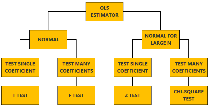
We also denote:

We now explain how to derive tests about the coefficients of the normal linear regression model.

It can be proved (see the lecture about the normal linear regression model ) that the assumption of conditional normality implies that:

How the acceptance region is determined depends not only on the desired size of the test , but also on whether the test is:

one-tailed (only one of the two things, i.e., either smaller or larger, is possible).

For more details on how to determine the acceptance region, see the glossary entry on critical values .

The F test is one-tailed .

A critical value in the right tail of the F distribution is chosen so as to achieve the desired size of the test.

Then, the null hypothesis is rejected if the F statistics is larger than the critical value.

In this section we explain how to perform hypothesis tests about the coefficients of a linear regression model when the OLS estimator is asymptotically normal.

As we have shown in the lecture on the properties of the OLS estimator , in several cases (i.e., under different sets of assumptions) it can be proved that:

These two properties are used to derive the asymptotic distribution of the test statistics used in hypothesis testing.

The test can be either one-tailed or two-tailed . The same comments made for the t-test apply here.

Like the F test, also the Chi-square test is usually one-tailed .

The desired size of the test is achieved by appropriately choosing a critical value in the right tail of the Chi-square distribution.

The null is rejected if the Chi-square statistics is larger than the critical value.

Want to learn more about regression analysis? Here are some suggestions:

R squared of a linear regression ;

Gauss-Markov theorem ;

Generalized Least Squares ;

Multicollinearity ;

Dummy variables ;

Selection of linear regression models

Partitioned regression ;

Ridge regression .

How to cite

Please cite as:

Taboga, Marco (2021). "Linear regression - Hypothesis testing", Lectures on probability theory and mathematical statistics. Kindle Direct Publishing. Online appendix. https://www.statlect.com/fundamentals-of-statistics/linear-regression-hypothesis-testing.

Most of the learning materials found on this website are now available in a traditional textbook format.

• F distribution
• Beta distribution
• Conditional probability
• Central Limit Theorem
• Binomial distribution
• Mean square convergence
• Delta method
• Almost sure convergence
• Mathematical tools
• Fundamentals of probability
• Probability distributions
• Asymptotic theory
• Fundamentals of statistics
• About Statlect
• Cookies, privacy and terms of use
• Loss function
• Almost sure
• Type I error
• Precision matrix
• Integrable variable
• To enhance your privacy,
• we removed the social buttons,
• but don't forget to share .

Simple Linear Regression

Simple linear regression #.

RStudio: RMarkdown , Quarto

Father & son data #

Pearson’s height data #.

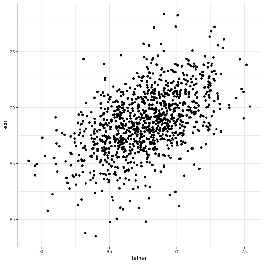
An example of simple linear regression model .

Breakdown of terms:

regression model : a model for the mean of a response given features

linear : model of the mean is linear in parameters of interest

simple : only a single feature

Slicewise model #

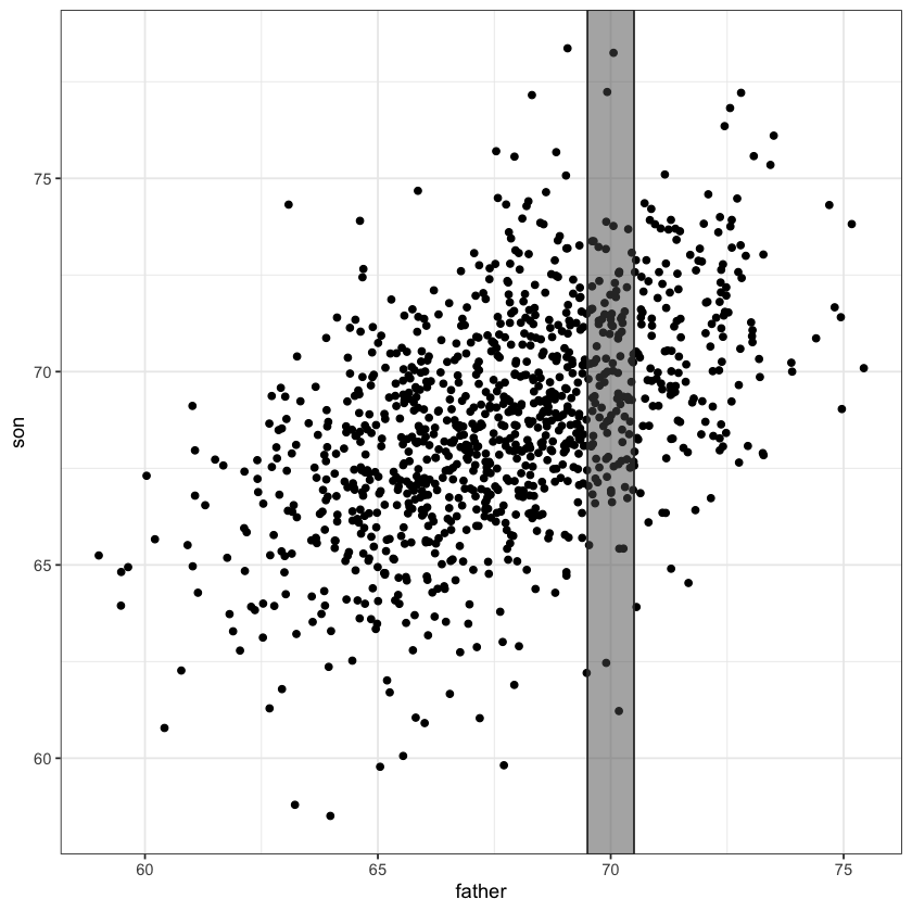
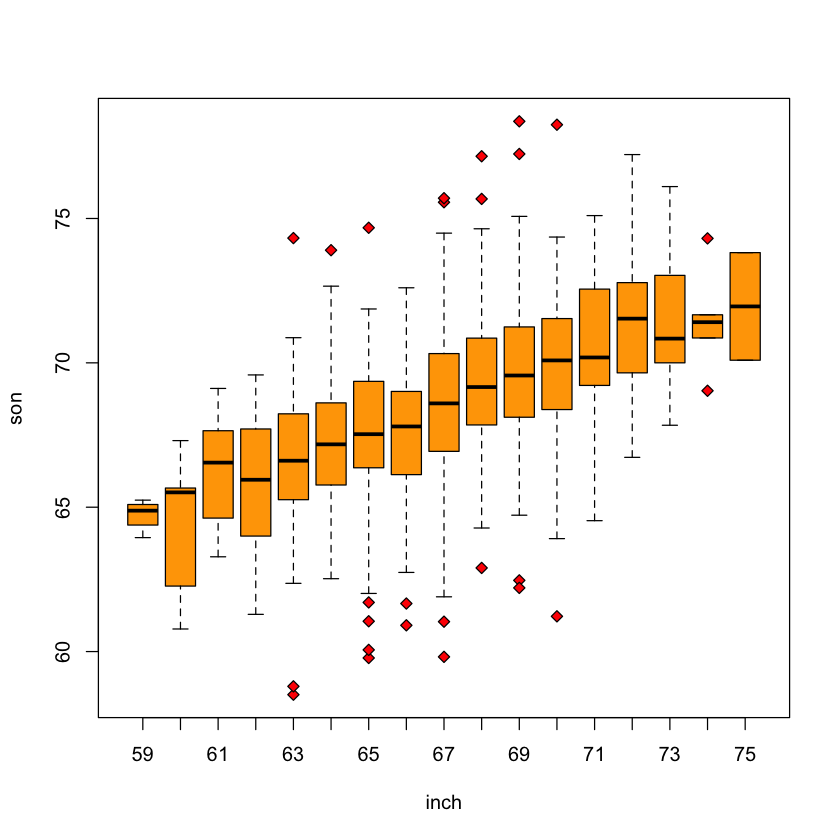
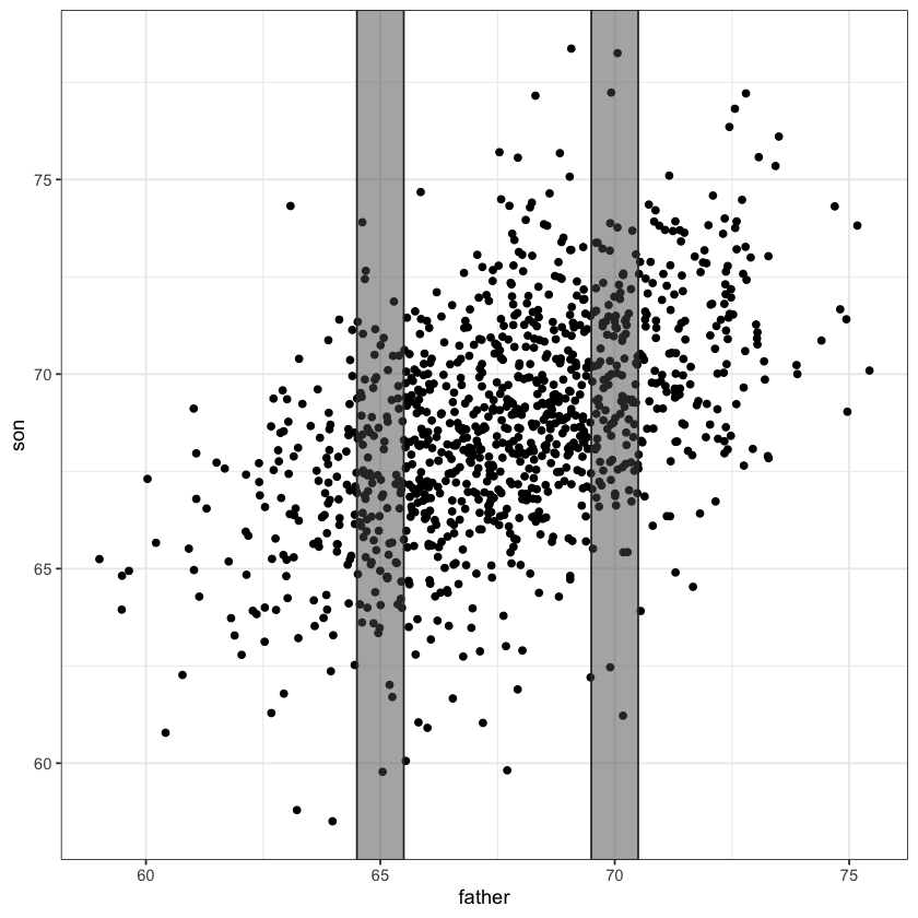
A simple linear regression model fits a line through the above scatter plot by modelling slices .

Conditional means #

The average height of sons whose height fell within our slice [69.5,79.5] is about 69.8 inches.

This height varies by slice…

At 65 inches it’s about 67.2 inches:

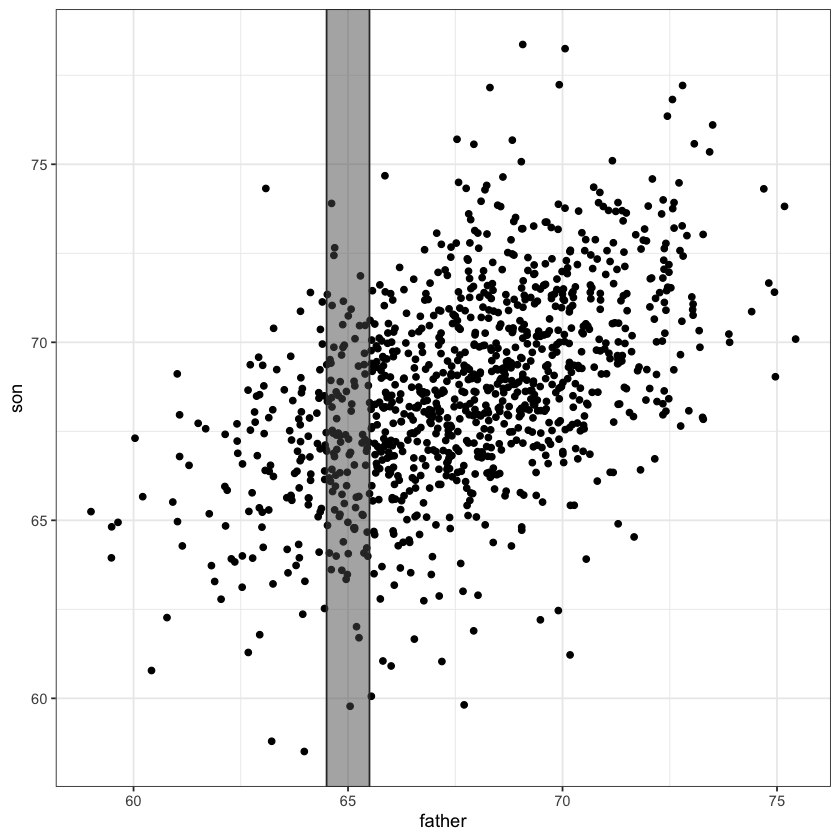
Multiple samples model ( longevity example) #

We’ve seen this slicewise model before: error in each slice the same.

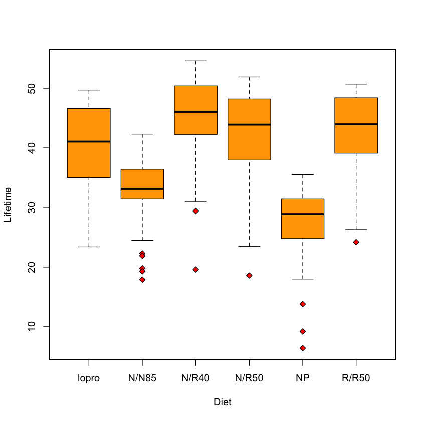
Regression as slicewise model #

In longevity model: no relation between the means in each slice! We needed to use a parameter for each Diet …

Regression model says that the mean in slice father is

This ties together all (father, son) points in the scatterplot.

Chooses \((\beta_0, \beta_1)\) by jointly modeling the mean in each slice…

Height data as slices #

What is a “regression” model? #

Model of the relationships between some covariates / predictors / features and an outcome .

A regression model is a model of the average outcome given the covariates .

Mathematical formulation #

For height data: a mathematical model:

\(f\) describes how mean of son varies with father

\(\varepsilon\) is the random variation within the slice.

Linear regression models #

A linear regression model says that the function \(f\) is a sum (linear combination) of functions of father .

Simple linear regression model:

Parameters of \(f\) are \((\beta_0, \beta_1)\)

Could also be a sum (linear combination) of fixed functions of father :

Statistical model #

Symbol \(Y\) usually used for outcomes, \(X\) for covariates…

Model: $ \( Y_i = \underbrace{\beta_0 + \beta_1 X_i}_{\text{regression equation}} + \underbrace{\varepsilon_i}_{\text{error}}\) $

where \(\varepsilon_i \sim N(0, \sigma^2)\) are independent.

This specifies a distribution for the \(Y\) ’s given the \(X\) ’s, i.e. it is a statistical model .

Regression equation #

The regression equation is our slicewise model.

Formally, this is a model of the conditional mean function

Book uses the notation \(\mu\{Y|X\}\) .

Fitting the model #

We will be using least squares regression. This measures the goodness of fit of a line by the sum of squared errors, \(SSE\) .

Least squares regression chooses the line that minimizes $ \( SSE(\beta_0, \beta_1) = \sum_{i=1}^n (Y_i - \beta_0 - \beta_1 \cdot X_i)^2.\) $

In principle, we might measure goodness of fit differently: $ \( SAD(\beta_0, \beta_1) = \sum_{i=1}^n |Y_i - \beta_0 - \beta_1 \cdot X_i|.\) $

For some other loss function \(L\) we might try to minimize $ \( L(\beta_0,\beta_1) = \sum_{i=1}^n L(Y_i-\beta_0-\beta_1\cdot X_i) \) $

Why least squares? #

With least squares, the minimizers have explicit formulae – not so important with today’s computer power.

Resulting formulae are linear in the outcome \(Y\) . This is important for inferential reasons. For only predictive power, this is also not so important.

If assumptions are correct, then this is maximum likelihood estimation .

Statistical theory tells us the maximum likelihood estimators (MLEs) are generally good estimators.

Choice of loss function #

Suppose we try to minimize squared error over \(\mu\) :

We know (by calculus) that the minimizer is the sample mean.

If we minimize absolute error over \(\mu\)

We know (similarly by calculus) that the minimizer(s) is (are) the sample median(s).

Visualizing the loss function #

Let’s take some a random scatter plot and view the loss function.

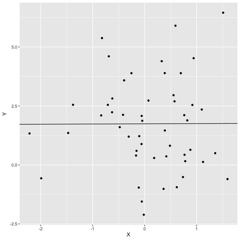
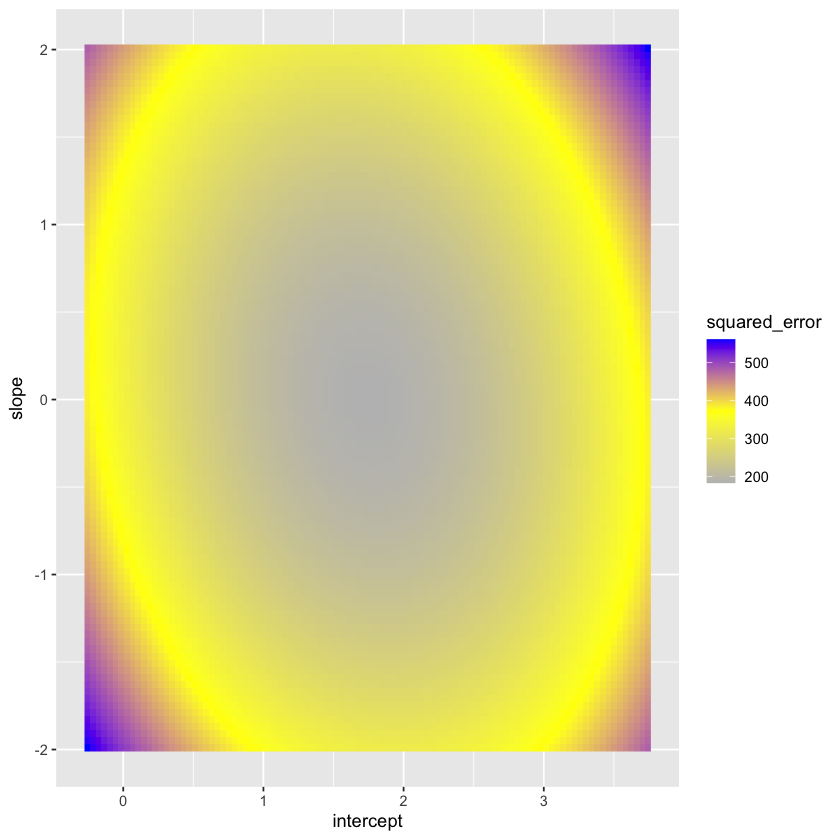
Let’s plot the loss as a function of the parameters. Note that the true intercept is 1.5 while the true slope is 0.1.

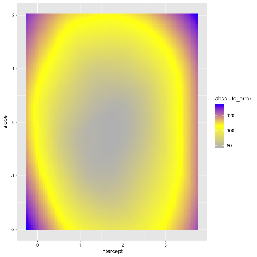
Let’s contrast this with the sum of absolute errors.

Geometry of least squares #

Some things to note:

Minimizing sum of squares is the same as finding the point in the X,1 plane closest to \(Y\) .

The total dimension of the space is 1078.

The dimension of the plane is 2-dimensional.

The axis marked “ \(\perp\) ” should be thought of as \((n-2)\) dimensional, or, 1076 in this case.

Least squares #

The (squared) lengths of the above vectors are important quantities in what follows.

Important lengths #

There are three to note: $ \( \begin{aligned} SSE &= \sum_{i=1}^n(Y_i - \widehat{Y}_i)^2 = \sum_{i=1}^n (Y_i - \widehat{\beta}_0 - \widehat{\beta}_1 X_i)^2 \\ SSR &= \sum_{i=1}^n(\overline{Y} - \widehat{Y}_i)^2 = \sum_{i=1}^n (\overline{Y} - \widehat{\beta}_0 - \widehat{\beta}_1 X_i)^2 \\ SST &= \sum_{i=1}^n(Y_i - \overline{Y})^2 = SSE + SSR \\ \end{aligned} \) $

An important summary of the fit is the ratio $ \( \begin{aligned} R^2 &= \frac{SSR}{SST} \\ &= 1 - \frac{SSE}{SST} \\ &= \widehat{Cor}(\pmb{X},\pmb{Y})^2. \end{aligned} \) $

Measures how much variability in \(Y\) is explained by \(X\) .

Case study A: data suggesting the Big Bang #

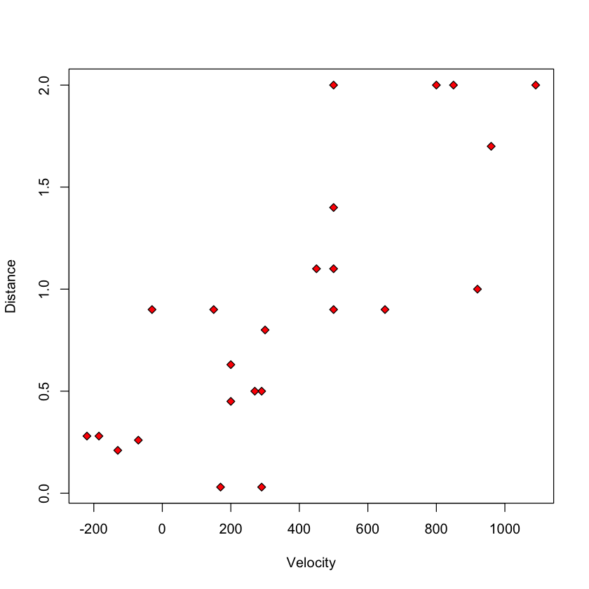
Let’s fit the linear regression model.

Let’s look at the summary :

Hubble’s model #

Hubble’s theory of the Big Bang suggests that the correct slicewise (i.e. regression) model is

To fit without an intercept

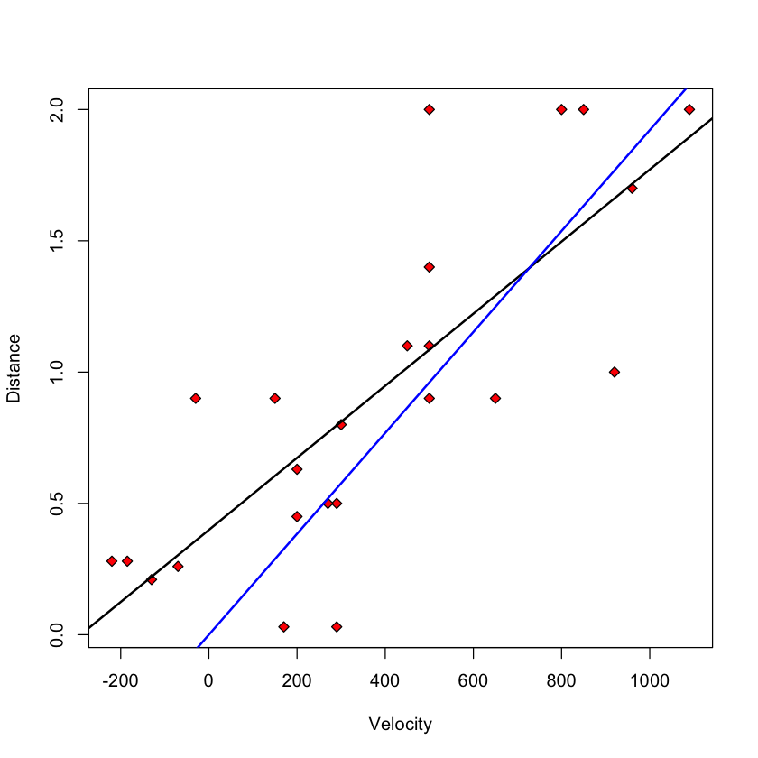
Least squares estimators #

There are explicit formulae for the least squares estimators, i.e. the minimizers of the error sum of squares.

For the slope, \(\hat{\beta}_1\) , it can be shown that $ \( \widehat{\beta}_1 = \frac{\sum_{i=1}^n(X_i - \overline{X})(Y_i - \overline{Y} )}{\sum_{i=1}^n (X_i-\overline{X})^2} = \frac{\widehat{Cov}(X,Y)}{\widehat{Var}( X)}.\) $

Knowing the slope estimate, the intercept estimate can be found easily: $ \( \widehat{\beta}_0 = \overline{Y} - \widehat{\beta}_1 \cdot \overline{ X}.\) $

Example: big_bang #

• 0.399170439725205
• 0.00137240753172474

Estimate of \(\sigma^2\) #

The estimate most commonly used is $ \( \begin{aligned} \hat{\sigma}^2 &= \frac{1}{n-2} \sum_{i=1}^n (Y_i - \hat{\beta}_0 - \hat{\beta}_1 X_i)^2 \\ & = \frac{SSE}{n-2} \\ &= MSE \end{aligned} \) $

We’ll use the common practice of replacing the quantity \(SSE(\hat{\beta}_0,\hat{\beta}_1)\) , i.e. the minimum of this function, with just \(SSE\) .

The term MSE above refers to mean squared error: a sum of squares divided by its degrees of freedom . The degrees of freedom of SSE , the error sum of squares is therefore \(n-2\) .

We divide by \(n-2\) because some calculations tell us: $ \( \frac{\hat{\sigma}^2}{\sigma^2} \sim \frac{\chi^2_{n-2}}{n-2} \) \( where the right hand side denotes a *chi-squared* distribution with \) n-2$ degrees of freedom.

Dividing by \(n-2\) gives an unbiased estimate of \(\sigma^2\) (assuming our modeling assumptions are correct).

Inference for the simple linear regression model #

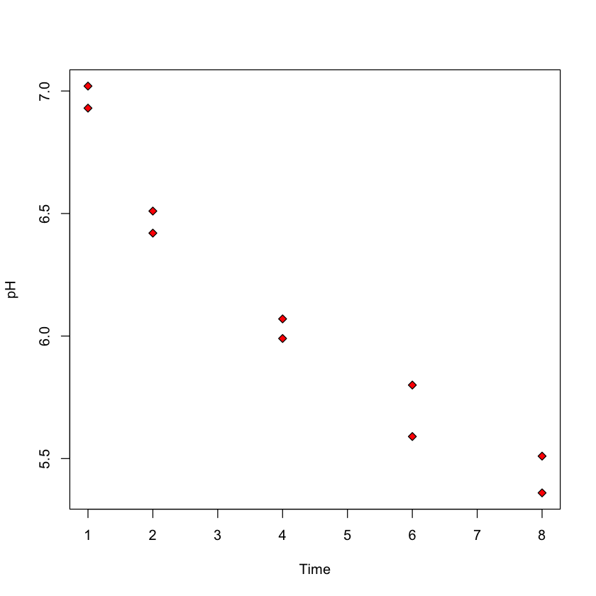
Case study b: predicting ph based on time after slaughter #.

In this study, researches fixed \(X\) ( Time ) before measuring \(Y\) ( pH )

Ultimate goal: how long after slaughter is pH around 6?

Inference for \(\beta_0\) or \(\beta_1\) #

Recall our model $ \( Y_i = \beta_0 + \beta_1 X_i + \varepsilon_i,\) \( errors \) \varepsilon_i \( are independent \) N(0, \sigma^2)$.

In our heights example, we might want to now if there really is a linear association between \({\tt son}=Y\) and \({\tt father}=X\) . This can be answered with a hypothesis test of the null hypothesis \(H_0:\beta_1=0\) . This assumes the model above is correct, AND \(\beta_1=0\) .

Alternatively, we might want to have a range of values that we can be fairly certain \(\beta_1\) lies within. This is a confidence interval for \(\beta_1\) .

A mathematical aside #

Let \(L\) be the subspace of \(\mathbb{R}^n\) spanned \(\pmb{1}=(1, \dots, 1)\) and \({X}=(X_1, \dots, X_n)\) .

We can decompose \(Y\) as

In our model, \(\mu=\beta_0 \pmb{1} + \beta_1 {X} \in L\) so that

Our assumption that \(\varepsilon_i\) ’s are independent \(N(0,\sigma^2)\) tells us that: \({e}\) and \(\widehat{{Y}}\) are independent; \(\widehat{\sigma}^2 = \|{e}\|^2 / (n-2) \sim \sigma^2 \cdot \chi^2_{n-2} / (n-2)\) .

Setup for inference #

All of this implies

The other quantity we need is the standard error or SE of \(\hat{\beta}_1\) :

Testing \(H_0:\beta_1=\beta_1^0\) #

Suppose we want to test that \(\beta_1\) is some pre-specified value, \(\beta_1^0\) (this is often 0: i.e. is there a linear association)

Under \(H_0:\beta_1=\beta_1^0\)

Reject \(H_0:\beta_1=\beta_1^0\) if \(|T| > t_{n-2, 1-\alpha/2}\) .

Let’s perform this test for the Big Bang data.

We see that R performs our \(t\) -test in the second row of the Coefficients table.

It is clear that Distance is correlated with Velocity .

There seems to be some flaw in Hubble’s theory: we reject \(H_0:\beta_0=0\) at level 5%: \(p\) -value is 0.0028!

Why reject for large |T|? #

Logic is the same as other \(t\) tests: observing a large \(|T|\) is unlikely if \(\beta_1 = \beta_1^0\) (i.e. if \(H_0\) were true). \(\implies\) it is reasonable to conclude that \(H_0\) is false.

Common to report \(p\) -value: $ \(\mathbb{P}(|T_{n-2}| > |T|_{obs}) = 2 \cdot \mathbb{P} (T_{n-2} > |T_{obs}|)\) $

Confidence interval for regression parameters #

Applying the above to the parameter \(\beta_1\) yields a confidence interval of the form

Earlier, we computed \(SE(\hat{\beta}_1)\) using this formula

with \((a_0,a_1) = (0, 1)\) .

We also need to find the quantity \(t_{n-2,1-\alpha/2}\) . This is defined by

In R , this is computed by the function qt .

We will not need to use these explicit formulae all the time, as R has some built in functions to compute confidence intervals.

Predicting the mean #

Once we have estimated a slope \((\hat{\beta}_1)\) and an intercept \((\hat{\beta}_0)\) , we can predict the height of the son born to a father of any particular height by the plugging-in the height of the new father, \(F_{new}\) into our regression equation:

Confidence interval for the average height of sons born to a father of height \(F_{new}=70\) (or maybe \(65\) ) inches:

Computing \(SE(\hat{\beta}_0 + 70 \cdot \hat{\beta}_1)\) #

We use the previous formula

with \((a_0, a_1) = (1, 70)\) .

Plugging in

As \(n\) grows (taking a larger sample), \(SE(\hat{\beta}_0 + 70 \hat{\beta}_1)\) should shrink to 0. Why?

Forecasting intervals #

Can we find an interval that covers the height of a particular son knowing only that her father’s height as 70 inches?

Must cover the variability of the new random variation \(\implies\) it must be at least as wide as \(\sigma\) .

With so much data in our heights example, this 90% interval will have width roughly \(2 \cdot 1.96 \cdot \hat{\sigma}\)

• 8.01555526222726
• 8.18982582776275

Actual width will depend on how accurately we have estimated \((\beta_0, \beta_1)\) as well as \(\hat{\sigma}\) .

The final interval is $ \( \hat{\beta}_0 + \hat{\beta}_1 \cdot 70 \pm t_{n-2, 1-\alpha/2} \cdot SE(\hat{\beta}_0 + \hat{\beta}_1 \cdot 70 + \varepsilon_{\text{new}}). \) $

User Preferences

Content preview.

Arcu felis bibendum ut tristique et egestas quis:

• Ut enim ad minim veniam, quis nostrud exercitation ullamco laboris
• Duis aute irure dolor in reprehenderit in voluptate
• Excepteur sint occaecat cupidatat non proident

Keyboard Shortcuts

6.4 - the hypothesis tests for the slopes.

At the beginning of this lesson, we translated three different research questions pertaining to heart attacks in rabbits ( Cool Hearts dataset ) into three sets of hypotheses we can test using the general linear F -statistic. The research questions and their corresponding hypotheses are:

Hypotheses 1

Is the regression model containing at least one predictor useful in predicting the size of the infarct?

• \(H_{0} \colon \beta_{1} = \beta_{2} = \beta_{3} = 0\)
• \(H_{A} \colon\) At least one \(\beta_{j} ≠ 0\) (for j = 1, 2, 3)

Hypotheses 2

Is the size of the infarct significantly (linearly) related to the area of the region at risk?

• \(H_{0} \colon \beta_{1} = 0 \)
• \(H_{A} \colon \beta_{1} \ne 0 \)

Hypotheses 3

(Primary research question) Is the size of the infarct area significantly (linearly) related to the type of treatment upon controlling for the size of the region at risk for infarction?

• \(H_{0} \colon \beta_{2} = \beta_{3} = 0\)
• \(H_{A} \colon \) At least one \(\beta_{j} ≠ 0\) (for j = 2, 3)

Let's test each of the hypotheses now using the general linear F -statistic:

\(F^*=\left(\dfrac{SSE(R)-SSE(F)}{df_R-df_F}\right) \div \left(\dfrac{SSE(F)}{df_F}\right)\)

To calculate the F -statistic for each test, we first determine the error sum of squares for the reduced and full models — SSE ( R ) and SSE ( F ), respectively. The number of error degrees of freedom associated with the reduced and full models — \(df_{R}\) and \(df_{F}\), respectively — is the number of observations, n , minus the number of parameters, p , in the model. That is, in general, the number of error degrees of freedom is n - p . We use statistical software, such as Minitab's F -distribution probability calculator, to determine the P -value for each test.

Testing all slope parameters equal 0 Section  

To answer the research question: "Is the regression model containing at least one predictor useful in predicting the size of the infarct?" To do so, we test the hypotheses:

• \(H_{0} \colon \beta_{1} = \beta_{2} = \beta_{3} = 0 \)
• \(H_{A} \colon\) At least one \(\beta_{j} \ne 0 \) (for j = 1, 2, 3)

The full model

The full model is the largest possible model — that is, the model containing all of the possible predictors. In this case, the full model is:

\(y_i=(\beta_0+\beta_1x_{i1}+\beta_2x_{i2}+\beta_3x_{i3})+\epsilon_i\)

The error sum of squares for the full model, SSE ( F ), is just the usual error sum of squares, SSE , that appears in the analysis of variance table. Because there are 4 parameters in the full model, the number of error degrees of freedom associated with the full model is \(df_{F} = n - 4\).

The reduced model

The reduced model is the model that the null hypothesis describes. Because the null hypothesis sets each of the slope parameters in the full model equal to 0, the reduced model is:

\(y_i=\beta_0+\epsilon_i\)

The reduced model suggests that none of the variations in the response y is explained by any of the predictors. Therefore, the error sum of squares for the reduced model, SSE ( R ), is just the total sum of squares, SSTO , that appears in the analysis of variance table. Because there is only one parameter in the reduced model, the number of error degrees of freedom associated with the reduced model is \(df_{R} = n - 1 \).

Upon plugging in the above quantities, the general linear F -statistic:

\(F^*=\dfrac{SSE(R)-SSE(F)}{df_R-df_F} \div \dfrac{SSE(F)}{df_F}\)

becomes the usual " overall F -test ":

\(F^*=\dfrac{SSR}{3} \div \dfrac{SSE}{n-4}=\dfrac{MSR}{MSE}\)

That is, to test \(H_{0}\) : \(\beta_{1} = \beta_{2} = \beta_{3} = 0 \), we just use the overall F -test and P -value reported in the analysis of variance table:

Analysis of Variance

Regression equation.

Inf = - 0.135 + 0.613 Area - 0.2435 X2 - 0.0657 X3

There is sufficient evidence ( F = 16.43, P < 0.001) to conclude that at least one of the slope parameters is not equal to 0.

In general, to test that all of the slope parameters in a multiple linear regression model are 0, we use the overall F -test reported in the analysis of variance table.

Testing one slope parameter is 0 Section  

Now let's answer the second research question: "Is the size of the infarct significantly (linearly) related to the area of the region at risk?" To do so, we test the hypotheses:

Again, the full model is the model containing all of the possible predictors:

The error sum of squares for the full model, SSE ( F ), is just the usual error sum of squares, SSE . Alternatively, because the three predictors in the model are \(x_{1}\), \(x_{2}\), and \(x_{3}\), we can denote the error sum of squares as SSE (\(x_{1}\), \(x_{2}\), \(x_{3}\)). Again, because there are 4 parameters in the model, the number of error degrees of freedom associated with the full model is \(df_{F} = n - 4 \).

Because the null hypothesis sets the first slope parameter, \(\beta_{1}\), equal to 0, the reduced model is:

\(y_i=(\beta_0+\beta_2x_{i2}+\beta_3x_{i3})+\epsilon_i\)

Because the two predictors in the model are \(x_{2}\) and \(x_{3}\), we denote the error sum of squares as SSE (\(x_{2}\), \(x_{3}\)). Because there are 3 parameters in the model, the number of error degrees of freedom associated with the reduced model is \(df_{R} = n - 3\).

The general linear statistic:

simplifies to:

\(F^*=\dfrac{SSR(x_1|x_2, x_3)}{1}\div \dfrac{SSE(x_1,x_2, x_3)}{n-4}=\dfrac{MSR(x_1|x_2, x_3)}{MSE(x_1,x_2, x_3)}\)

Getting the numbers from the Minitab output:

we determine that the value of the F -statistic is:

\(F^* = \dfrac{SSR(x_1 \vert x_2, x_3)}{1} \div \dfrac{SSE(x_1, x_2, x_3)}{28} = \dfrac{0.63742}{0.01946}=32.7554\)

The P -value is the probability — if the null hypothesis were true — that we would get an F -statistic larger than 32.7554. Comparing our F -statistic to an F -distribution with 1 numerator degree of freedom and 28 denominator degrees of freedom, Minitab tells us that the probability is close to 1 that we would observe an F -statistic smaller than 32.7554:

F distribution with 1 DF in Numerator and 28 DF in denominator

Therefore, the probability that we would get an F -statistic larger than 32.7554 is close to 0. That is, the P -value is < 0.001. There is sufficient evidence ( F = 32.8, P < 0.001) to conclude that the size of the infarct is significantly related to the size of the area at risk after the other predictors x2 and x3 have been taken into account.

But wait a second! Have you been wondering why we couldn't just use the slope's t -statistic to test that the slope parameter, \(\beta_{1}\), is 0? We can! Notice that the P -value ( P < 0.001) for the t -test ( t * = 5.72):

Coefficients

is the same as the P -value we obtained for the F -test. This will always be the case when we test that only one slope parameter is 0. That's because of the well-known relationship between a t -statistic and an F -statistic that has one numerator degree of freedom:

\(t_{(n-p)}^{2}=F_{(1, n-p)}\)

For our example, the square of the t -statistic, 5.72, equals our F -statistic (within rounding error). That is:

\(t^{*2}=5.72^2=32.72=F^*\)

So what have we learned in all of this discussion about the equivalence of the F -test and the t -test? In short:

Compare the output obtained when \(x_{1}\) = Area is entered into the model last :

Inf = - 0.135 - 0.2435 X2 - 0.0657 X3 + 0.613 Area

to the output obtained when \(x_{1}\) = Area is entered into the model first :

The t -statistic and P -value are the same regardless of the order in which \(x_{1}\) = Area is entered into the model. That's because — by its equivalence to the F -test — the t -test for one slope parameter adjusts for all of the other predictors included in the model.

• We can use either the F -test or the t -test to test that only one slope parameter is 0. Because the t -test results can be read right off of the Minitab output, it makes sense that it would be the test that we'll use most often.
• But, we have to be careful with our interpretations! The equivalence of the t -test to the F -test has taught us something new about the t -test. The t -test is a test for the marginal significance of the \(x_{1}\) predictor after the other predictors \(x_{2}\) and \(x_{3}\) have been taken into account. It does not test for the significance of the relationship between the response y and the predictor \(x_{1}\) alone.

Testing a subset of slope parameters is 0 Section  

Finally, let's answer the third — and primary — research question: "Is the size of the infarct area significantly (linearly) related to the type of treatment upon controlling for the size of the region at risk for infarction?" To do so, we test the hypotheses:

• \(H_{0} \colon \beta_{2} = \beta_{3} = 0 \)
• \(H_{A} \colon\) At least one \(\beta_{j} \ne 0 \) (for j = 2, 3)

Because the null hypothesis sets the second and third slope parameters, \(\beta_{2}\) and \(\beta_{3}\), equal to 0, the reduced model is:

\(y_i=(\beta_0+\beta_1x_{i1})+\epsilon_i\)

The ANOVA table for the reduced model is:

Because the only predictor in the model is \(x_{1}\), we denote the error sum of squares as SSE (\(x_{1}\)) = 0.8793. Because there are 2 parameters in the model, the number of error degrees of freedom associated with the reduced model is \(df_{R} = n - 2 = 32 – 2 = 30\).

\begin{align} F^*&=\dfrac{SSE(R)-SSE(F)}{df_R-df_F} \div\dfrac{SSE(F)}{df_F}\\&=\dfrac{0.8793-0.54491}{30-28} \div\dfrac{0.54491}{28}\\&= \dfrac{0.33439}{2} \div 0.01946\\&=8.59.\end{align}

Alternatively, we can calculate the F-statistic using a partial F-test :

\begin{align}F^*&=\dfrac{SSR(x_2, x_3|x_1)}{2}\div \dfrac{SSE(x_1,x_2, x_3)}{n-4}\\&=\dfrac{MSR(x_2, x_3|x_1)}{MSE(x_1,x_2, x_3)}.\end{align}

To conduct the test, we regress y = InfSize on \(x_{1}\) = Area and \(x_{2}\) and \(x_{3 }\)— in order (and with "Sequential sums of squares" selected under "Options"):

Inf = - 0.135 + 0.613 Area - 0.2435 X2 - 0.0657 X3

yielding SSR (\(x_{2}\) | \(x_{1}\)) = 0.31453, SSR (\(x_{3}\) | \(x_{1}\), \(x_{2}\)) = 0.01981, and MSE = 0.54491/28 = 0.01946. Therefore, the value of the partial F -statistic is:

\begin{align} F^*&=\dfrac{SSR(x_2, x_3|x_1)}{2}\div \dfrac{SSE(x_1,x_2, x_3)}{n-4}\\&=\dfrac{0.31453+0.01981}{2}\div\dfrac{0.54491}{28}\\&= \dfrac{0.33434}{2} \div 0.01946\\&=8.59,\end{align}

which is identical (within round-off error) to the general F-statistic above. The P -value is the probability — if the null hypothesis were true — that we would observe a partial F -statistic more extreme than 8.59. The following Minitab output:

F distribution with 2 DF in Numerator and 28 DF in denominator

tells us that the probability of observing such an F -statistic that is smaller than 8.59 is 0.9988. Therefore, the probability of observing such an F -statistic that is larger than 8.59 is 1 - 0.9988 = 0.0012. The P -value is very small. There is sufficient evidence ( F = 8.59, P = 0.0012) to conclude that the type of cooling is significantly related to the extent of damage that occurs — after taking into account the size of the region at risk.

Summary of MLR Testing Section  

For the simple linear regression model, there is only one slope parameter about which one can perform hypothesis tests. For the multiple linear regression model, there are three different hypothesis tests for slopes that one could conduct. They are:

• Hypothesis test for testing that all of the slope parameters are 0.
• Hypothesis test for testing that a subset — more than one, but not all — of the slope parameters are 0.
• Hypothesis test for testing that one slope parameter is 0.

We have learned how to perform each of the above three hypothesis tests. Along the way, we also took two detours — one to learn about the " general linear F-test " and one to learn about " sequential sums of squares. " As you now know, knowledge about both is necessary for performing the three hypothesis tests.

The F -statistic and associated p -value in the ANOVA table is used for testing whether all of the slope parameters are 0. In most applications, this p -value will be small enough to reject the null hypothesis and conclude that at least one predictor is useful in the model. For example, for the rabbit heart attacks study, the F -statistic is (0.95927/(4–1)) / (0.54491/(32–4)) = 16.43 with p -value 0.000.

To test whether a subset — more than one, but not all — of the slope parameters are 0, there are two equivalent ways to calculate the F-statistic:

• Use the general linear F-test formula by fitting the full model to find SSE(F) and fitting the reduced model to find SSE(R) . Then the numerator of the F-statistic is (SSE(R) – SSE(F)) / ( \(df_{R}\) – \(df_{F}\)) .
• Alternatively, use the partial F-test formula by fitting only the full model but making sure the relevant predictors are fitted last and "sequential sums of squares" have been selected. Then the numerator of the F-statistic is the sum of the relevant sequential sums of squares divided by the sum of the degrees of freedom for these sequential sums of squares. The denominator of the F -statistic is the mean squared error in the ANOVA table.

For example, for the rabbit heart attacks study, the general linear F-statistic is ((0.8793 – 0.54491) / (30 – 28)) / (0.54491 / 28) = 8.59 with p -value 0.0012. Alternatively, the partial F -statistic for testing the slope parameters for predictors \(x_{2}\) and \(x_{3}\) using sequential sums of squares is ((0.31453 + 0.01981) / 2) / (0.54491 / 28) = 8.59.

To test whether one slope parameter is 0, we can use an F -test as just described. Alternatively, we can use a t -test, which will have an identical p -value since in this case, the square of the t -statistic is equal to the F -statistic. For example, for the rabbit heart attacks study, the F -statistic for testing the slope parameter for the Area predictor is (0.63742/1) / (0.54491/(32–4)) = 32.75 with p -value 0.000. Alternatively, the t -statistic for testing the slope parameter for the Area predictor is 0.613 / 0.107 = 5.72 with p -value 0.000, and \(5.72^{2} = 32.72\).

Incidentally, you may be wondering why we can't just do a series of individual t-tests to test whether a subset of the slope parameters is 0. For example, for the rabbit heart attacks study, we could have done the following:

• Fit the model of y = InfSize on \(x_{1}\) = Area and \(x_{2}\) and \(x_{3}\) and use an individual t-test for \(x_{3}\).
• If the test results indicate that we can drop \(x_{3}\) then fit the model of y = InfSize on \(x_{1}\) = Area and \(x_{2}\) and use an individual t-test for \(x_{2}\).

The problem with this approach is we're using two individual t-tests instead of one F-test, which means our chance of drawing an incorrect conclusion in our testing procedure is higher. Every time we do a hypothesis test, we can draw an incorrect conclusion by:

• rejecting a true null hypothesis, i.e., make a type I error by concluding the tested predictor(s) should be retained in the model when in truth it/they should be dropped; or
• failing to reject a false null hypothesis, i.e., make a type II error by concluding the tested predictor(s) should be dropped from the model when in truth it/they should be retained.

Thus, in general, the fewer tests we perform the better. In this case, this means that wherever possible using one F-test in place of multiple individual t-tests is preferable.

Hypothesis tests for the slope parameters Section  

The problems in this section are designed to review the hypothesis tests for the slope parameters, as well as to give you some practice on models with a three-group qualitative variable (which we'll cover in more detail in Lesson 8). We consider tests for:

• whether one slope parameter is 0 (for example, \(H_{0} \colon \beta_{1} = 0 \))
• whether a subset (more than one but less than all) of the slope parameters are 0 (for example, \(H_{0} \colon \beta_{2} = \beta_{3} = 0 \) against the alternative \(H_{A} \colon \beta_{2} \ne 0 \) or \(\beta_{3} \ne 0 \) or both ≠ 0)
• whether all of the slope parameters are 0 (for example, \(H_{0} \colon \beta_{1} = \beta_{2} = \beta_{3}\) = 0 against the alternative \(H_{A} \colon \) at least one of the \(\beta_{i}\) is not 0)

(Note the correct specification of the alternative hypotheses for the last two situations.)

Sugar beets study

A group of researchers was interested in studying the effects of three different growth regulators ( treat , denoted 1, 2, and 3) on the yield of sugar beets (y = yield , in pounds). They planned to plant the beets in 30 different plots and then randomly treat 10 plots with the first growth regulator, 10 plots with the second growth regulator, and 10 plots with the third growth regulator. One problem, though, is that the amount of available nitrogen in the 30 different plots varies naturally, thereby giving a potentially unfair advantage to plots with higher levels of available nitrogen. Therefore, the researchers also measured and recorded the available nitrogen (\(x_{1}\) = nit , in pounds/acre) in each plot. They are interested in comparing the mean yields of sugar beets subjected to the different growth regulators after taking into account the available nitrogen. The Sugar Beets dataset contains the data from the researcher's experiment.

Preliminary Work

The plot shows a similar positive linear trend within each treatment category, which suggests that it is reasonable to formulate a multiple regression model that would place three parallel lines through the data.

Because the qualitative variable treat distinguishes between the three treatment groups (1, 2, and 3), we need to create two indicator variables, \(x_{2}\) and \(x_{3}\), say, to fit a linear regression model to these data. The new indicator variables should be defined as follows:

Use Minitab's Calc >> Make Indicator Variables command to create the new indicator variables in your worksheet

Minitab creates an indicator variable for each treatment group but we can only use two, for treatment groups 1 and 2 in this case (treatment group 3 is the reference level in this case).

Then, if we assume the trend in the data can be summarized by this regression model:

\(y_{i} = \beta_{0}\) + \(\beta_{1}\)\(x_{1}\) + \(\beta_{2}\)\(x_{2}\) + \(\beta_{3}\)\(x_{3}\) + \(\epsilon_{i}\)

where \(x_{1}\) = nit and \(x_{2}\) and \(x_{3}\) are defined as above, what is the mean response function for plots receiving treatment 3? for plots receiving treatment 1? for plots receiving treatment 2? Are the three regression lines that arise from our formulated model parallel? What does the parameter \(\beta_{2}\) quantify? And, what does the parameter \(\beta_{3}\) quantify?

The fitted equation from Minitab is Yield = 84.99 + 1.3088 Nit - 2.43 \(x_{2}\) - 2.35 \(x_{3}\), which means that the equations for each treatment group are:

• Group 1: Yield = 84.99 + 1.3088 Nit - 2.43(1) = 82.56 + 1.3088 Nit
• Group 2: Yield = 84.99 + 1.3088 Nit - 2.35(1) = 82.64 + 1.3088 Nit
• Group 3: Yield = 84.99 + 1.3088 Nit

The three estimated regression lines are parallel since they have the same slope, 1.3088.

The regression parameter for \(x_{2}\) represents the difference between the estimated intercept for treatment 1 and the estimated intercept for reference treatment 3.

The regression parameter for \(x_{3}\) represents the difference between the estimated intercept for treatment 2 and the estimated intercept for reference treatment 3.

Testing whether all of the slope parameters are 0

\(H_0 \colon \beta_1 = \beta_2 = \beta_3 = 0\) against the alternative \(H_A \colon \) at least one of the \(\beta_i\) is not 0.

\(F=\dfrac{SSR(X_1,X_2,X_3)\div3}{SSE(X_1,X_2,X_3)\div(n-4)}=\dfrac{MSR(X_1,X_2,X_3)}{MSE(X_1,X_2,X_3)}\)

\(F = \dfrac{\frac{16039.5}{3}}{\frac{1078.0}{30-4}} = \dfrac{5346.5}{41.46} = 128.95\)

Since the p -value for this F -statistic is reported as 0.000, we reject \(H_{0}\) in favor of \(H_{A}\) and conclude that at least one of the slope parameters is not zero, i.e., the regression model containing at least one predictor is useful in predicting the size of sugar beet yield.

Tests for whether one slope parameter is 0

\(H_0 \colon \beta_1= 0\) against the alternative \(H_A \colon \beta_1 \ne 0\)

t -statistic = 19.60, p -value = 0.000, so we reject \(H_{0}\) in favor of \(H_{A}\) and conclude that the slope parameter for \(x_{1}\) = nit is not zero, i.e., sugar beet yield is significantly linearly related to the available nitrogen (controlling for treatment).

\(F=\dfrac{SSR(X_1|X_2,X_3)\div1}{SSE(X_1,X_2,X_3)\div(n-4)}=\dfrac{MSR(X_1|X_2,X_3)}{MSE(X_1,X_2,X_3)}\)

Use the Minitab output to calculate the value of this F statistic. Does the value you obtain equal \(t^{2}\), the square of the t -statistic as we might expect?

\(F-statistic= \dfrac{\frac{15934.5}{1}}{\frac{1078.0}{30-4}} = \dfrac{15934.5}{41.46} = 384.32\), which is the same as \(19.60^{2}\).

Because \(t^{2}\) will equal the partial F -statistic whenever you test for whether one slope parameter is 0, it makes sense to just use the t -statistic and P -value that Minitab displays as a default. But, note that we've just learned something new about the meaning of the t -test in the multiple regression setting. It tests for the ("marginal") significance of the \(x_{1}\) predictor after \(x_{2}\) and \(x_{3}\) have already been taken into account.

Tests for whether a subset of the slope parameters is 0

\(H_0 \colon \beta_2=\beta_3= 0\) against the alternative \(H_A \colon \beta_2 \ne 0\) or \(\beta_3 \ne 0\) or both \(\ne 0\).

\(F=\dfrac{SSR(X_2,X_3|X_1)\div2}{SSE(X_1,X_2,X_3)\div(n-4)}=\dfrac{MSR(X_2,X_3|X_1)}{MSE(X_1,X_2,X_3)}\)

\(F = \dfrac{\frac{10.4+27.5}{2}}{\frac{1078.0}{30-4}} = \dfrac{18.95}{41.46} = 0.46\).

F distribution with 2 DF in Numerator and 26 DF in denominator

p-value \(= 1-0.363677 = 0.636\), so we fail to reject \(H_{0}\) in favor of \(H_{A}\) and conclude that we cannot rule out \(\beta_2 = \beta_3 = 0\), i.e., there is no significant difference in the mean yields of sugar beets subjected to the different growth regulators after taking into account the available nitrogen.

Note that the sequential mean square due to regression, MSR(\(X_{2}\),\(X_{3}\)|\(X_{1}\)), is obtained by dividing the sequential sum of square by its degrees of freedom (2, in this case, since two additional predictors \(X_{2}\) and \(X_{3}\) are considered). Use the Minitab output to calculate the value of this F statistic, and use Minitab to get the associated P -value. Answer the researcher's question at the \(\alpha= 0.05\) level.

• Prompt Library
• DS/AI Trends
• Stats Tools
• Interview Questions
• Generative AI
• Machine Learning
• Deep Learning

Linear regression hypothesis testing: Concepts, Examples

In relation to machine learning , linear regression is defined as a predictive modeling technique that allows us to build a model which can help predict continuous response variables as a function of a linear combination of explanatory or predictor variables. While training linear regression models, we need to rely on hypothesis testing in relation to determining the relationship between the response and predictor variables. In the case of the linear regression model, two types of hypothesis testing are done. They are T-tests and F-tests . In other words, there are two types of statistics that are used to assess whether linear regression models exist representing response and predictor variables. They are t-statistics and f-statistics. As data scientists , it is of utmost importance to determine if linear regression is the correct choice of model for our particular problem and this can be done by performing hypothesis testing related to linear regression response and predictor variables. Many times, it is found that these concepts are not very clear with a lot many data scientists. In this blog post, we will discuss linear regression and hypothesis testing related to t-statistics and f-statistics . We will also provide an example to help illustrate how these concepts work.

Table of Contents

What are linear regression models?

A linear regression model can be defined as the function approximation that represents a continuous response variable as a function of one or more predictor variables. While building a linear regression model, the goal is to identify a linear equation that best predicts or models the relationship between the response or dependent variable and one or more predictor or independent variables.

There are two different kinds of linear regression models. They are as follows:

• Simple or Univariate linear regression models : These are linear regression models that are used to build a linear relationship between one response or dependent variable and one predictor or independent variable. The form of the equation that represents a simple linear regression model is Y=mX+b, where m is the coefficients of the predictor variable and b is bias. When considering the linear regression line, m represents the slope and b represents the intercept.
• Multiple or Multi-variate linear regression models : These are linear regression models that are used to build a linear relationship between one response or dependent variable and more than one predictor or independent variable. The form of the equation that represents a multiple linear regression model is Y=b0+b1X1+ b2X2 + … + bnXn, where bi represents the coefficients of the ith predictor variable. In this type of linear regression model, each predictor variable has its own coefficient that is used to calculate the predicted value of the response variable.

While training linear regression models, the requirement is to determine the coefficients which can result in the best-fitted linear regression line. The learning algorithm used to find the most appropriate coefficients is known as least squares regression . In the least-squares regression method, the coefficients are calculated using the least-squares error function. The main objective of this method is to minimize or reduce the sum of squared residuals between actual and predicted response values. The sum of squared residuals is also called the residual sum of squares (RSS). The outcome of executing the least-squares regression method is coefficients that minimize the linear regression cost function .

The residual e of the ith observation is represented as the following where [latex]Y_i[/latex] is the ith observation and [latex]\hat{Y_i}[/latex] is the prediction for ith observation or the value of response variable for ith observation.

[latex]e_i = Y_i – \hat{Y_i}[/latex]

The residual sum of squares can be represented as the following:

[latex]RSS = e_1^2 + e_2^2 + e_3^2 + … + e_n^2[/latex]

The least-squares method represents the algorithm that minimizes the above term, RSS.

Once the coefficients are determined, can it be claimed that these coefficients are the most appropriate ones for linear regression? The answer is no. After all, the coefficients are only the estimates and thus, there will be standard errors associated with each of the coefficients.  Recall that the standard error is used to calculate the confidence interval in which the mean value of the population parameter would exist. In other words, it represents the error of estimating a population parameter based on the sample data. The value of the standard error is calculated as the standard deviation of the sample divided by the square root of the sample size. The formula below represents the standard error of a mean.

[latex]SE(\mu) = \frac{\sigma}{\sqrt(N)}[/latex]

Thus, without analyzing aspects such as the standard error associated with the coefficients, it cannot be claimed that the linear regression coefficients are the most suitable ones without performing hypothesis testing. This is where hypothesis testing is needed . Before we get into why we need hypothesis testing with the linear regression model, let’s briefly learn about what is hypothesis testing?

Train a Multiple Linear Regression Model using R

Before getting into understanding the hypothesis testing concepts in relation to the linear regression model, let’s train a multi-variate or multiple linear regression model and print the summary output of the model which will be referred to, in the next section. 

The data used for creating a multi-linear regression model is BostonHousing which can be loaded in RStudioby installing mlbench package. The code is shown below:

install.packages(“mlbench”) library(mlbench) data(“BostonHousing”)

Once the data is loaded, the code shown below can be used to create the linear regression model.

attach(BostonHousing) BostonHousing.lm <- lm(log(medv) ~ crim + chas + rad + lstat) summary(BostonHousing.lm)

Executing the above command will result in the creation of a linear regression model with the response variable as medv and predictor variables as crim, chas, rad, and lstat. The following represents the details related to the response and predictor variables:

• log(medv) : Log of the median value of owner-occupied homes in USD 1000’s
• crim : Per capita crime rate by town
• chas : Charles River dummy variable (= 1 if tract bounds river; 0 otherwise)
• rad : Index of accessibility to radial highways
• lstat : Percentage of the lower status of the population

The following will be the output of the summary command that prints the details relating to the model including hypothesis testing details for coefficients (t-statistics) and the model as a whole (f-statistics) 

Hypothesis tests & Linear Regression Models

Hypothesis tests are the statistical procedure that is used to test a claim or assumption about the underlying distribution of a population based on the sample data. Here are key steps of doing hypothesis tests with linear regression models:

• Hypothesis formulation for T-tests: In the case of linear regression, the claim is made that there exists a relationship between response and predictor variables, and the claim is represented using the non-zero value of coefficients of predictor variables in the linear equation or regression model. This is formulated as an alternate hypothesis. Thus, the null hypothesis is set that there is no relationship between response and the predictor variables . Hence, the coefficients related to each of the predictor variables is equal to zero (0). So, if the linear regression model is Y = a0 + a1x1 + a2x2 + a3x3, then the null hypothesis for each test states that a1 = 0, a2 = 0, a3 = 0 etc. For all the predictor variables, individual hypothesis testing is done to determine whether the relationship between response and that particular predictor variable is statistically significant based on the sample data used for training the model. Thus, if there are, say, 5 features, there will be five hypothesis tests and each will have an associated null and alternate hypothesis.
• Hypothesis formulation for F-test : In addition, there is a hypothesis test done around the claim that there is a linear regression model representing the response variable and all the predictor variables. The null hypothesis is that the linear regression model does not exist . This essentially means that the value of all the coefficients is equal to zero. So, if the linear regression model is Y = a0 + a1x1 + a2x2 + a3x3, then the null hypothesis states that a1 = a2 = a3 = 0.
• F-statistics for testing hypothesis for linear regression model : F-test is used to test the null hypothesis that a linear regression model does not exist, representing the relationship between the response variable y and the predictor variables x1, x2, x3, x4 and x5. The null hypothesis can also be represented as x1 = x2 = x3 = x4 = x5 = 0. F-statistics is calculated as a function of sum of squares residuals for restricted regression (representing linear regression model with only intercept or bias and all the values of coefficients as zero) and sum of squares residuals for unrestricted regression (representing linear regression model). In the above diagram, note the value of f-statistics as 15.66 against the degrees of freedom as 5 and 194. 
• Evaluate t-statistics against the critical value/region : After calculating the value of t-statistics for each coefficient, it is now time to make a decision about whether to accept or reject the null hypothesis. In order for this decision to be made, one needs to set a significance level, which is also known as the alpha level. The significance level of 0.05 is usually set for rejecting the null hypothesis or otherwise. If the value of t-statistics fall in the critical region, the null hypothesis is rejected. Or, if the p-value comes out to be less than 0.05, the null hypothesis is rejected.
• Evaluate f-statistics against the critical value/region : The value of F-statistics and the p-value is evaluated for testing the null hypothesis that the linear regression model representing response and predictor variables does not exist. If the value of f-statistics is more than the critical value at the level of significance as 0.05, the null hypothesis is rejected. This means that the linear model exists with at least one valid coefficients. 
• Draw conclusions : The final step of hypothesis testing is to draw a conclusion by interpreting the results in terms of the original claim or hypothesis. If the null hypothesis of one or more predictor variables is rejected, it represents the fact that the relationship between the response and the predictor variable is not statistically significant based on the evidence or the sample data we used for training the model. Similarly, if the f-statistics value lies in the critical region and the value of the p-value is less than the alpha value usually set as 0.05, one can say that there exists a linear regression model.

Why hypothesis tests for linear regression models?

The reasons why we need to do hypothesis tests in case of a linear regression model are following:

• By creating the model, we are establishing a new truth (claims) about the relationship between response or dependent variable with one or more predictor or independent variables. In order to justify the truth, there are needed one or more tests. These tests can be termed as an act of testing the claim (or new truth) or in other words, hypothesis tests.
• One kind of test is required to test the relationship between response and each of the predictor variables (hence, T-tests)
• Another kind of test is required to test the linear regression model representation as a whole. This is called F-test.

While training linear regression models, hypothesis testing is done to determine whether the relationship between the response and each of the predictor variables is statistically significant or otherwise. The coefficients related to each of the predictor variables is determined. Then, individual hypothesis tests are done to determine whether the relationship between response and that particular predictor variable is statistically significant based on the sample data used for training the model. If at least one of the null hypotheses is rejected, it represents the fact that there exists no relationship between response and that particular predictor variable. T-statistics is used for performing the hypothesis testing because the standard deviation of the sampling distribution is unknown. The value of t-statistics is compared with the critical value from the t-distribution table in order to make a decision about whether to accept or reject the null hypothesis regarding the relationship between the response and predictor variables. If the value falls in the critical region, then the null hypothesis is rejected which means that there is no relationship between response and that predictor variable. In addition to T-tests, F-test is performed to test the null hypothesis that the linear regression model does not exist and that the value of all the coefficients is zero (0). Learn more about the linear regression and t-test in this blog – Linear regression t-test: formula, example .

Recent Posts

• Model Parallelism vs Data Parallelism: Examples - April 11, 2024
• Model Complexity & Overfitting in Machine Learning: How to Reduce - April 10, 2024
• 6 Game-Changing Features of ChatGPT’s Latest Upgrade - April 9, 2024

Ajitesh Kumar

One response.

Very informative

Leave a Reply Cancel reply

Your email address will not be published. Required fields are marked *

• Search for:
• Excellence Awaits: IITs, NITs & IIITs Journey

ChatGPT Prompts (250+)

• Generate Design Ideas for App
• Expand Feature Set of App
• Create a User Journey Map for App
• Generate Visual Design Ideas for App
• Generate a List of Competitors for App
• Model Parallelism vs Data Parallelism: Examples
• Model Complexity & Overfitting in Machine Learning: How to Reduce
• 6 Game-Changing Features of ChatGPT’s Latest Upgrade
• Self-Prediction vs Contrastive Learning: Examples
• Free IBM Data Sciences Courses on Coursera

Data Science / AI Trends

• • Prepend any arxiv.org link with talk2 to load the paper into a responsive chat application
• • Custom LLM and AI Agents (RAG) On Structured + Unstructured Data - AI Brain For Your Organization
• • Guides, papers, lecture, notebooks and resources for prompt engineering
• • Common tricks to make LLMs efficient and stable
• • Machine learning in finance

Free Online Tools

• Create Scatter Plots Online for your Excel Data
• Histogram / Frequency Distribution Creation Tool
• Online Pie Chart Maker Tool
• Z-test vs T-test Decision Tool
• Independent samples t-test calculator

Recent Comments

I found it very helpful. However the differences are not too understandable for me

Very Nice Explaination. Thankyiu very much,

in your case E respresent Member or Oraganization which include on e or more peers?

Such a informative post. Keep it up

Thank you....for your support. you given a good solution for me.

• Privacy Policy

How to Write and Test Statistical Hypotheses in Simple Linear Regression

We need to develop hypotheses when conducting research. A hypothesis is a provisional assumption or statement of the research. The hypothesis needs to be proven, whether true or false, through the research process.

To prove the hypothesis, we need to test the hypothesis to see whether the proposed hypothesis is accepted or rejected. On the other hand, researchers still use linear regression tools very often.

Therefore, on this occasion, Kanda Data will discuss how to write and test statistical hypotheses in simple linear regression. In principle, research hypotheses need to be derived into statistical hypotheses.

We can test whether the research hypothesis is accepted or rejected through this statistical hypothesis. Before discussing further, in hypothesis testing, we need to recognize the assumptions/statements, often referred to as the null hypothesis.

In developing statistical hypotheses, the null hypothesis is the hypothesis being tested. The notation H 0 often expresses the null hypothesis.

In principle, if statistical hypothesis testing states that H 0 is rejected, it can be interpreted that we accept the alternative hypothesis. Alternative hypotheses are often expressed with the notation H 1 or Ha.

Mini Research Example

Suppose we conduct a mini-research to determine how price influences the volume of clothes sold. Because the ratio data scale measured both variables for this study, we can use a simple linear regression analysis.

Why do we use simple linear regression? The answer is that the regression equation used only consists of one independent variable and one dependent variable.

In this simple linear regression analysis, it is necessary to test the assumptions to obtain the best linear unbiased estimator. Test assumptions that need to be fulfilled, for example, normality, non-heteroscedasticity, and linearity tests.

How to Write a Statistical Hypothesis

Statistical hypotheses on simple linear regression can be written more simply and easily. This statistical hypothesis is a representation of your research hypothesis.

Based on the example of the mini-research that I conveyed earlier, the research hypothesis that we can propose is that price significantly affects the volume of clothing sales.

The research hypotheses can then be compiled into statistical hypotheses as follows:

H 0 : b = 0; clothing prices have no significant effect on clothing sales volume

H 1 : b ≠ 0; clothing prices have a significant effect on clothing sales volume

Determine the error significance level (alpha)

In testing the statistical hypothesis that has been compiled, the next step is to determine the level of significance of the error (alpha). Determination of the alpha significance level can be different for several types of fields of science.

For experimental research in general, the alpha significance level is set at 5% or 1%. Meanwhile, survey research can determine the alpha significance level of up to 10%.

Finding t-value

The t value in simple linear regression can be calculated manually or using statistical software. For manual t-value calculations, you can read my article entitled: “ How to find the variance, standard error, and t-value in simple linear regression .”

If you determine the t-value using statistical software, the t-value will generally be in the coefficient table in the regression output. The advantage of using statistical software is that in addition to obtaining the t-value, we can also directly find out the p-value of alpha.

Hypothesis test

Statistical hypothesis testing can use the one-tailed test and the two-tailed test. Based on the previous statistical hypothesis, I used a two-tailed statistical test.

In testing the hypothesis, it can be determined in two ways: comparing the t-value with the t-table and comparing the p-value of the regression output with the alpha significance level.

The statistical hypothesis testing criteria for the 1st method are:

If t-value ≤ t-table, H 0 is accepted (H 1 is rejected)

If t-value > t-table, H 0 is rejected (H 1 is accepted)

Because we are using a two-way test, the value of t can be positive and can be negative. Thus, Ho is rejected if t-value>t-table or -(t-value)<-(t-table), and vice versa.

Furthermore, for the statistical hypothesis testing criteria for the 2nd method, namely:

If p-value ≥ alpha, H 0 is accepted (H 1 is rejected)

If p-value < alpha, H 0 is rejected (H 1 is accepted)

For example, the t value of the regression output is -6.604 with a p-value <0.05, it can be concluded that we reject H 0 (accept H 1 ). Therefore, we can conclude that clothing price has a significant effect on the volume of clothing sales.

Well, that’s our discussion this time. I hope it will be beneficial for all of us. See you in the following article!

• how to construct a hypothesis
• Hypothesis testing
• hypothesis testing in linear regression
• Hypothesis tests in simple linear regression
• linear regression hypothesis tests
• simple linear regression

Understanding the Essence of the Difference Between Descriptive Statistics and Inferential Statistics in Research

Can nominal scale data be analyzed using regression analysis, data that cannot be transformed using natural logarithm (ln).

[…] To read other articles that discuss hypothesis testing, you can read my articles entitled: “How to write and test statistical hypotheses in simple linear regression” and “How does high variance affect hypothesis testing in linear […]

LEAVE A REPLY Cancel reply

Save my name, email, and website in this browser for the next time I comment.

Most Popular

Reasons why likert scale variables need to undergo validity and reliability testing, understanding the difference between residual and error in regression analysis, the difference between simultaneous equation system model and linear regression equation, understanding the importance of the coefficient of determination in linear regression analysis, understanding the essence of assumption testing in linear regression analysis: prominent differences between cross-sectional data and time series data, understanding the difference between paired t-test and wilcoxon test in statistics, recent comments.

Statistics Made Easy

Understanding the t-Test in Linear Regression

Linear regression is used to quantify the relationship between a predictor variable and a response variable.

Whenever we perform linear regression, we want to know if there is a statistically significant relationship between the predictor variable and the response variable.

We test for significance by performing a t-test for the regression slope. We use the following null and alternative hypothesis for this t-test:

• H 0 : β 1 = 0 (the slope is equal to zero)
• H A : β 1 ≠ 0 (the slope is not equal to zero)

We then calculate the test statistic as follows:

• t = b  / SE b
• b : coefficient estimate
• SE b : standard error of the coefficient estimate

If the p-value that corresponds to t is less than some threshold (e.g. α = .05) then we reject the null hypothesis and conclude that there is a statistically significant relationship between the predictor variable and the response variable.

The following example shows how to perform a t-test for a linear regression model in practice.

Example: Performing a t-Test for Linear Regression

Suppose a professor wants to analyze the relationship between hours studied and exam score received for 40 of his students.

He performs simple linear regression using hours studied as the predictor variable and exam score received as the response variable.

The following table shows the results of the regression model:

To determine if hours studied has a statistically significant relationship with final exam score, we can perform a t-test.

We use the following null and alternative hypothesis for this t-test:

• H 0 : β 1 = 0 (the slope for hours studied is equal to zero)
• H A : β 1 ≠ 0 (the slope for hours studied is not equal to zero)
• t = 1.117 / 1.025

The p-value that corresponds to t = 1.089 with df = n-2 = 40 – 2 = 38 is 0.283 .

Note that we can also use the T Score to P Value Calculator to calculate this p-value:

Since this p-value is not less than .05, we fail to reject the null hypothesis.

This means that hours studied does not have a statistically significant relationship between final exam score.

Additional Resources

The following tutorials offer additional information about linear regression:

Introduction to Simple Linear Regression Introduction to Multiple Linear Regression How to Interpret Regression Coefficients How to Interpret the F-Test of Overall Significance in Regression

Published by Zach

Leave a reply cancel reply.

Your email address will not be published. Required fields are marked *