hypothesis on deforestation

• Search Menu
• Advance Articles
• Author Guidelines
• Submission Site
• Open Access
• Self-Archiving Policy
• Why Submit?
• About Journal of Forestry
• About Society of American Foresters
• Editorial Board
• Advertising & Corporate Services
• Journals Career Network
• Journals on Oxford Academic
• Books on Oxford Academic

Article Contents

Addressing the complexities and impacts of deforestation.

• < Previous

Addressing the Complexities and Impacts of Deforestation

• Article contents
• Figures & tables
• Supplementary Data

John Stanturf, Addressing the Complexities and Impacts of Deforestation, Journal of Forestry , Volume 115, Issue 4, July 2017, Pages 319–320, https://doi.org/10.5849/jof.2016-069

• Permissions Icon Permissions

Deforestation, the removal of forest canopy and conversion to another land use, has engendered significant international efforts to stop or reverse loss of tree cover. Seen today, deforestation would appear to be an issue of tropical forests even though the cumulative loss of forestland over the last 5,000 years is estimated globally at 1.8 billion ha. In Global Deforestation , Runyan and D'Odorico provide a thorough analysis of the literature, and to say that their book is broad in scope is perhaps an understatement. It is multidisciplinary, addressing perspectives from the biophysical as well as social sciences and examines processes at multiple spatial and temporal scales. The book addresses the complexity of deforestation, including considering the benefits of deforestation (mostly private and short-term) as well as the costs (social and long-term). A further strength of the book is that effects examined go beyond the deforested area, for example, including the potential regional climatic effects of deforestation and afforestation. This comprehensive approach, which should appeal to researchers and students, may seem a bit too “academic” for managers. The summaries of main points provided by the authors within and at the end of chapters, however, should appeal to all readers.

Global Deforestation is a relatively short book, comprising just six chapters but well referenced, and some figures are reproduced in color at the end. It begins with an introduction to the drivers of deforestation, including a historical perspective that describes the trajectory of clearing and in some cases recovery by region. Potential future drivers (principally meeting food security and dietary preferences of an expanding human population) are introduced in Chapter 1 (“Introduction: Patterns and Drivers”) and explored in-depth in Chapter 6 (“Synthesis and Future Impacts of Deforestation”). The intervening chapters address impacts of deforestation on hydrology and climate, biogeochemistry, ecological irreversibility, and, of course, economic impacts and drivers. Each chapter on impacts has a similar structure, first describing underlying processes (or baseline conditions) and then the effects of deforestation on important aspects of a process. For example, Chapter 2, “Hydrologic and Climatic Impacts,” has sections describing precipitation and forest canopies and infiltration and runoff generation before launching into the effects of deforestation on the hydrologic responses of flood dynamics and water yields. Also considered in this chapter are the effects of forests on groundwater and deforestation on wetlands, evaporation and transpiration and the effects of forests on precipitation and microclimate, and the effects of deforestation on large-scale climate. The chapter effectively presents a minireview of the importance of forests in climate change discussions that venture beyond carbon sequestration.

The chapter on irreversibility and ecosystem impacts ties the previous chapters to current thinking on disturbance and ecosystem resilience and resistance. Specific feedbacks that modify resource availability are presented in terms of operating principles, geographic extent, available observational evidence, modeling techniques to address the complexity, and management implications. The situations considered are potentially where deforestation leads to conditions that cannot support forest vegetation, such as following landslides, wildfire, exposure to freezing events, or increased soil salinity. These are cases where an abrupt transition to a seemingly irreversible state, with loss of economic and ecological functions, has significant implications for restoration efforts. Unfortunately, the authors do not draw out these implications in greater detail; more on this later.

Chapter 5, “Economic Impacts and Drivers of Deforestation,” is where many authors would begin their story; to the credit of Runyan and D'Odorico, however, they lay the biophysical groundwork first before venturing into the very complex social context of land-use decisions. They use the framework that is well established in the literature of immediate (proximate) versus underlying (ultimate) causes and note that agricultural expansion is the primary cause of deforestation, although other factors such as road building that improves access to markets can determine the historical development of reduced forest cover in a region. Two paradoxes of importance to conservation and sustainable development emerge regarding improved agricultural productivity and secure tenure. First, agricultural intensification has been promoted as a way to reduce pressure on native forests (i.e., avoided deforestation). In actuality, yield increases and labor-saving technology may lead to increased deforestation because agriculture is more profitable. Second, insecure land tenure, typical of many areas in the tropics where deforestation is occurring, could lead a farmer to decline to invest in improvements or long-term investments such as forestry; thus, secure tenure could lead to greater emphasis on future benefits from value accumulated in timber. Conversely, secure property rights could induce the farmer to invest in agriculture and use the land as collateral for loans to cover the costs of improvement. In both instances, other sociocultural conditions play a role in which scenario plays out.

On the whole, Global Deforestation is a valuable addition to the literature on an important international issue of great interest to foresters. Although it may be slow going for some readers in parts due to the comprehensive treatment of technical issues, the brief summaries within some chapters and at the end of each provide needed rest from the details and helpful reminders of the larger picture. Considering the benefits to some people and costs to others makes the case that deforestation occurs for economic and social reasons and is not due to moral failure or ignorance. Reversing deforestation, therefore, requires addressing the immediate and underlying drivers, which is shown to be far from a simple task and one that requires more effort at multiple levels of society and not just in communities near tropical forests. I would be remiss as a reviewer if I couldn't identify two shortcomings. Even though the authors define deforestation clearly in the Introduction as involving long-term reduction of forest cover to below 10%, they still treat logging in several places as a general deforestation factor. This will be a burr under the saddle of most foresters. To their credit, the authors place relatively little emphasis on this, however. Finally, I would have appreciated the authors addressing current international efforts to address and reverse deforestation. Even though REDD+ is briefly mentioned, other efforts such as the Bonn Challenge to restore 150 million ha of forested landscapes by 2020 and 350 million ha by 2030 or the Convention on Biological Diversity Aichi Targets are ignored. Giving some insight into how to ensure these efforts are successful would have been a valuable conclusion to an interesting book.

Email alerts

Citing articles via.

• Recommend to Your Librarian
• Advertising and Corporate Services

Affiliations

• Online ISSN 1938-3746
• Print ISSN 0022-1201
• Copyright © 2024 Society of American Foresters
• About Oxford Academic
• Publish journals with us
• University press partners
• What we publish
• New features  
• Open access
• Institutional account management
• Rights and permissions
• Get help with access
• Accessibility
• Advertising
• Media enquiries
• Oxford University Press
• Oxford Languages
• University of Oxford

Oxford University Press is a department of the University of Oxford. It furthers the University's objective of excellence in research, scholarship, and education by publishing worldwide

• Copyright © 2024 Oxford University Press
• Cookie settings
• Cookie policy
• Privacy policy
• Legal notice

This Feature Is Available To Subscribers Only

Sign In or Create an Account

This PDF is available to Subscribers Only

For full access to this pdf, sign in to an existing account, or purchase an annual subscription.

Tropical Forestry Handbook pp 2987–3018 Cite as

Identifying the Causes of Tropical Deforestation: Meta-analysis to Test and Develop Economic Theory

• Stibniati Atmadja 3 &
• Erin Sills 4  
• Reference work entry

275 Accesses

2 Citations

This chapter discusses methods for summarizing and distilling lessons from the empirical economics literature on tropical forestry, giving particular attention to the method of meta-analysis (“the study of studies”) and to the topic of tropical deforestation. Meta-analysis can be used to take stock of the literature, test hypotheses about the effects of explanatory variables on a dependent variable, and predict the value of a dependent variable across space and time. We discuss previous reviews of the literature on deforestation and then illustrate how to test hypotheses with meta-analysis. Specifically, we examine the so-called “win-win” hypothesis that economic development is good for both people (resulting in higher incomes) and forests (resulting in lower rates of deforestation). Consistent with previous literature reviews, we find that the drivers of deforestation vary by region. However, we reject the win-win hypothesis in all regions: meta-analysis of the literature clearly shows that there are trade-offs between development and forest conservation. In Latin America, there is some evidence for the alternative hypothesis of an “environmental Kuznets curve” of deforestation. The meta-analysis also reveals possible publication biases, including different patterns of results in economics versus other publication outlets, which are important to keep in mind when drawing conclusions from the literature.

This is a preview of subscription content, log in via an institution .

Buying options

• Available as PDF
• Read on any device
• Instant download
• Own it forever
• Available as EPUB and PDF
• Durable hardcover edition
• Dispatched in 3 to 5 business days
• Free shipping worldwide - see info

Tax calculation will be finalised at checkout

Purchases are for personal use only

For an example, see the “SEED” database, available here: http://www.cgdev.org/publication/data-set-what-drives-deforestation-and-what-stops-it-meta-analysis-spatially-explicit

Nelson and Kennedy ( 2009 ) typify the economic approach to meta-analysis with their focus on statistical modeling decisions. In contrast, Rudel ( 2008 ) focuses more on the process of identifying and extracting data from the studies, arguing “that to carry out insightful and credible meta-analyses, researchers must address a set of recurring questions about (1) case study selection, (2) coding procedures, (3) variable selection, and (4) conjoint causation.”

This illustrates one possible way to search for publication bias. Ferretti-Gallon and Busch ( 2014 ) demonstrate another approach by comparing “results where a variable was the focus of a study vs. results of studies where that variable was included only as a control,” under the assumption that the first type of study would be less susceptible to bias against reporting statistically insignificant results. They note “that all four of the meta-variables for which the sign diverged based on whether or not the variable was the focus of the study were related to somewhat controversial or ideologically charged topics for which publication bias might be more suspected: community forestry, land tenure security, poverty, and rural income support.”

Angelsen A, Kaimowitz D (1999) Rethinking the causes of deforestation: lessons from economic models. World Bank Res Obs 14(1):73–98

Google Scholar  

Angelsen A, Rudel TK (2013) Designing and implementing effective REDD + policies: a forest transition approach. Rev Environ Econ Policy 7(1):91–113

Article   Google Scholar  

Asner GP, Loarie SR, Heyder U (2010) Combined effects of climate and land-use change on the future of humid tropical forests. Conserv Lett 3(6):395–403

Atmadja S (2003) Looking for a win-win situation: meta-analysis of deforestation and poverty. Master’s thesis, North Carolina State University, Raleigh

Atmadja S, Sills EO (2008) Deforestation and poverty: what is the consensus? Paper presented at the European Association of environmental and resource economists, Gothenburg, 25–28 Jun 2008

Barrio M, Loureiro ML (2010) A meta-analysis of contingent valuation forest studies. Ecol Econ 69(5):1023–1030

Beach RH, Pattanayak SK, Yang JC, Murray BC, Abt RC (2005) Econometric studies of non-industrial private forest management: a review and synthesis. For Policy Econ 7(3):261–281

Bergstrom JC, Taylor LO (2006) Using meta-analysis for benefits transfer: theory and practice. Ecol Econ 60(2):351–360

Blackman A, Rivera J (2010) Environmental certification and the global environment facility: STAP advisory document. Prepared on behalf of the scientific and technical advisory panel (STAP) of the global environment facility (GEF), Washington, DC

Bowler D, Buyung-Ali L, Healey JR, Jones JPG, Knight T, Pullin AS (2010) The evidence base of community forest management as a mechanism for supplying global environmental benefits and improving local welfare.? A STAP advisory document, Bangor University, Bangor

Brown K, Pearce D (eds) (1994) The causes of tropical deforestation: the economic and statistical analysis of factors giving rise to the loss of the tropical forests. University College London Press, London

Carson RT (2010) The environmental Kuznets curve: seeking empirical regularity and theoretical structure. Rev Environ Econ Policy 4(1):3–23

CEE (Collaboration for Environmental Evidence) (2014) Environmental evidence library of systematic reviews. Available from: http://www.environmentalevidence.org/completed-reviews

Choumert J, Combes Motel P, Dakpo HK (2013) Is the Environmental Kuznets Curve for deforestation a threatened theory? A meta-analysis of the literature. Ecol Econ 90:19–28

Collaboration for Environmental Evidence (2013) Guidelines for systematic review and evidence synthesis in environmental management. Version 4.2. Environmental evidence. www.environmentalevidence.org/Documents/Guidelines/Guidelines4.2.pdf . Accessed 15 Apr 2014

Dinda S (2004) Environmental Kuznets curve hypothesis: a survey. Ecol Econ 49(4):431–455

Dwan K, Altman DG, Arnaiz JA, Bloom J, Chan A-W, Cronin E, Decullier E, Easterbrook PJ, Elm EV, Gamble C, Ghersi D, Ioannidis JPA, Simes J, Williamson PR (2008) Systematic review of the empirical evidence of study publication bias and outcome reporting bias. PLoS One 3(8), e3081

Easterbrook PJ, Gopalan R, Berlin JA, Matthews DR (1991) Publication bias in clinical research. Lancet 337(8746):867–872

FAO (Food and Agriculture Organization) (2012) Global forest land-use change 1990–2005. FAO forestry paper #169. FAO, Rome

Ferretti-Gallon K, Busch J (2014) What drives deforestation and what stops it? A meta-analysis of spatially explicit econometric studies. Center for Global Development working paper 361. Washington, DC

Geist HJ, Lambin EF (2002) Proximate causes and underlying driving forces of tropical deforestation. BioScience 52(2):143–150

Geldmann J, Barnes M, Coad L, Craigie I, Hockings M, Burgess N (2013) Effectiveness of terrestrial protected areas in reducing biodiversity and habitat loss. CEE 10-007. Collaboration for Environmental Evidence

Geoghegan J, Villar SC, Klepeis P, Mendoza PM, Ogneva-Himmelberger Y, Chowdhury RR, Turner BL II, Vance C (2001) Modeling tropical deforestation in the southern Yucatan peninsular region: comparing survey and satellite data. Agr Ecosyst Environ 85(1):25–46

Gibson L, Lee TM, Koh LP, Brook BW, Gardner TA, Barlow J, Peres CA, Bradshaw CJA, Laurance WF, Lovejoy TE, Sodhi NS (2011) Primary forests are irreplaceable for sustaining tropical biodiversity. Nature 478(7369):378–381

Glass GV, McGaw B, Smith ML (1981) Meta-analysis in social research. Sage Publications, Beverly Hills

Grant MJ, Booth A (2009) A typology of reviews: an analysis of 14 review types and associated methodologies. Health Info Libr J 26(2):91–108

Article   PubMed   Google Scholar  

Gullison RE, Frumhoff PC, Canadell JG, Field CB, Nepstad DC, Hayhoe K, Avissar R, Curran LM, Friedlingstein P, Jones CD, Nobre C (2007) Tropical forests and climate policy. Science 316:985–986

Harris NL, Brown S, Hagen SC, Saatchi SS, Petrova S, Salas W, Hansen MC, Potapov PV, Lotsch A (2012) Baseline map of carbon emissions from deforestation in tropical regions. Science 336(6088):1573–1576

Hosonuma N, Herold M, De Sy V, De Fries RS, Brockhaus M, Verchot L, Angelsen A, Romijn E (2012) An assessment of deforestation and forest degradation drivers in developing countries. Environ Res Lett 7(4):044009

Kaimowitz D, Angelsen A (1998) Economic models of tropical deforestation: a review. CIFOR, Center for International Forestry Research, Bogor

Laurance WF (2007) Have we overstated the tropical biodiversity crisis? Trends Ecol Evol 22(2):65–70

Laurance WF, Sayer J, Cassman KG (2014) Agricultural expansion and its impacts on tropical nature. Trends Ecol Evol 29(2):107–116

Lewis JJ, Pattanayak SK (2012) Who adopts improved fuels and cookstoves? A systematic review. Environ Health Perspect 120(5):637

Article   PubMed   PubMed Central   Google Scholar  

Loomis JB, White DS (1996) Economic benefits of rare and endangered species: summary and meta-analysis. Ecol Econ 18(3):197–206

Miteva DA, Pattanayak SK, Ferraro PJ (2012) Evaluation of biodiversity policy instruments: what works and what doesn’t? Oxf Rev Econ Policy 28:69–92

Moher D, Liberati A, Tetzlaff J, Altman DG (2009) Preferred reporting items for systematic reviews and meta-analyses: the PRISMA statement. Ann Intern Med 151(4):264–269

Nelson JP, Kennedy PE (2009) The use (and abuse) of meta-analysis in environmental and natural resource economics: an assessment. Environ Resour Econ 42:345–377

Pattanayak SK, Mercer DE, Sills E, Yang JC (2003) Taking stock of agroforestry adoption studies. Agrofor Syst 57(3):173–186

Pfaff A, Amacher GS, Sills EO (2013) Realistic REDD: improving the forest impacts of domestic policies in different settings. Rev Environ Econ Policy 7(1):114–135

Robinson BE, Holland MB, Naughton-Treves L (2011) Does secure land tenure save forests? A review of the relationship between land tenure and tropical deforestation. CCAFS working paper. CCAFS, Copenhagen

Rudel T (2005) Tropical forests: regional paths of destruction and regeneration in the late 20th century. Columbia University Press, New York

Rudel TK, Flesher K, Bates D, Baptista S, Holmgren P (2000) Tropical deforestation literature: geographical and historical patterns. Unasylva 203(51):11–18

Rudel TK, Coomes OT, Moran E, Achard F, Angelsen A, Xu J, Lambin E (2005) Forest transitions: towards a global understanding of land use change. Glob Environ Chang 15(1):23–31

Rudel TK, Defries R, Asner GP, Laurance WF (2009) Changing drivers of deforestation and new opportunities for conservation. Conserv Biol 23(6):1396–1405

Samii C, Lisiecki M, Kulkarni P, Paler L, Chavis L (2014) Effects of Payment for Environmental Services (PES) on Deforestation and Poverty in Low and Middle Income Countries: a systematic review. CEE 13-015b. Collaboration for Environmental Evidence

Smith VK, Pattanayak SK, Van Houtven GL (2006) Structural benefit transfer: an example using VSL estimates. Ecol Econ 60(2):361–371

Tellis GJ (1988) The price elasticity of selective demand: a meta-analysis of economic models of sales. J Mark Res 25(4):331–341

Turner EH, Matthews AM, Linardatos E, Tell RA, Rosenthal R (2008) Selective publication of antidepressant trials and its influence on apparent efficacy. N Engl J Med 358:252–260

White H, Waddington H (2012) Why do we care about evidence synthesis? An introduction to the special issue on systematic reviews. J Dev Eff 4(3):351–358

Wolf FM (1986) Meta-analysis: quantitative methods for research synthesis, vol 59, Quantitative applications in the social sciences. Sage Publications, Beverly Hills

Book   Google Scholar  

Wunder S (2001) Poverty alleviation and tropical forests – what scope for synergies? World Dev 29(11):1817–1833

Wunder S, Wertz-Kanounnikoff S, Ferraro P (2010) PES and the GEF. Prepared on behalf of the scientific and technical advisory panel (STAP) of the global environment facility (GEF). Washington, DC

Zandersen M, Tol RS (2009) A meta-analysis of forest recreation values in Europe. J For Econ 15(1):109–130

List of Studies Included in Meta-analysis of Deforestation

Abizaid C, Coomes OT (2004) Land use and forest fallowing dynamics in seasonally dry tropical forests of the southern Yucatan Peninsula, Mexico. Land Use Policy 21:71–84

Aggrey N, Wambugu S, Karugia J, Wanga E (2010) An investigation of the poverty- environmental degradation nexus: a case study of Katonga Basin in Uganda. Res J Environ Earth Sci 2(2):82–88

Andersen LE (1996) The causes of deforestation in the Brazilian Amazon. J Environ Dev 5(3):309–328

Angelsen A, Katemansimba-Shitindi EF, Aarrestad J (1999) Why do farmers expand their land into forests? Theories and evidence from Tanzania. Environ Dev Econ 43(3):313–331

Antle JM, Heidebrink G (1995) Environment and development: theory and international evidence. Econ Dev Cult Chang 43(3):603–625

Araujo C, Bonjean CA, Combes J-L, Motel PC, Reis EJ (2010) Does land tenure insecurity drive deforestation in the Brazilian Amazon? Etudes et documents no. E 2010.13. CERDI, Clermont-Ferrand

Armenteras D, Rodriguez N, Retana J, Morales M (2011) Understanding deforestation in montane and lowland forests of the Colombian Andes. Reg Environ Chang 11(3):693–705

Austin K (2010a) The “Hamburger connection” as ecologically unequal exchange: a cross-national investigation of beef exports and deforestation in less-developed countries. Rural Sociol 75(2):270–299

Austin KF (2010b) Soybean exports and deforestation from a world-systems perspective: a cross-national investigation of comparative disadvantage. Sociol Q 51(3):511–536

Barbier EB (2004) Explaining agricultural land expansion and deforestation in developing countries. Am J Agric Econ 86(5):1347–1353

Barbier E, Burgess JC (2001) The economics of tropical deforestation. J Econ Surv 15(3):413–433

Basu A, Nayak NC (2011) Underlying causes of forest cover change in Odisha, India. For Policy Econ 13(7):563–569

Bawa KS, Dayanandan S (1997) Socioeconomic factors and tropical deforestation. Nature 386:582–583

Bhattarai M, Hammig M (2001) Institutions and the environmental Kuznets curve for deforestation: a crosscountry analysis for Latin America, Africa and Asia. World Dev 29(6):995–1010

Bhattarai M, Hammig M (2004) Governance, economic policy, and the environmental Kuznets curve for natural tropical forests. Environ Dev Econ 9:367–382

Blackman A, Rivera J (2010) Environmental certification and the global environment facility: STAP advisory document. Prepared on behalf of the Scientific and Technical Advisory Panel (STAP) of the Global Environment Facility (GEF), Washington, DC

Capistrano A (1994) Tropical forest depletion and the changing macroeconomy. In: Brown K, Pearce D (eds) The causes of tropical deforestation: the economic and statistical analysis of factors giving rise to the loss of the tropical forests. University College London Press, London, pp 1967–85

Capistrano AD, Kiker CF (1995) Macro-scale economic influences on tropical forest depletion. Ecol Econ 14:21–29

Caviglia-Harris JL (2004) Household production and forest clearing: the role of farming in the development of the Amazon. Environ Dev Econ 9(2):181–202

Caviglia-Harris J, Harris DW (2005) Examining the reliability of survey data with remote sensing and geographic information systems to improve deforestation modeling. Rev Reg Stud 35(2):187–205

Chakraborty M (1994) An analysis of the causes of deforestation in India. In: Brown K, Pearce D (eds) The causes of tropical deforestation: the economic and statistical analysis of factors giving rise to the loss of the tropical forests. University College London Press, London

Codjoe SNA, Dzanku FM (2009) Long-term determinants of deforestation in Ghana: the role of structural adjustment policies. Afr Dev Rev 21(3):558–588

Cropper M, Griffiths C (1994) The interaction of population growth and environmental quality. Am Econ Rev 84(2):250–254

Cropper M, Griffiths C, Mani M (1997) Roads, population pressures, and deforestation in Thailand, 1976–89. World Bank, Washington, DC

Culas RJ (2007) Deforestation and the environmental Kuznets curve: an institutional perspective. Ecol Econ 61(2–3):429–437

Culas R, Dutta D (2002) The underlying causes of deforestation and environmental Kuznets curve: a crosscountry analysis. In: Econometric Society of Australasia meeting (ESAM02), Queensland University of Technology, Brisbane, 7–10 Jul 2002.

Damette O, Delacote P (2011) Unsustainable timber harvesting, deforestation and the role of certification. Ecol Econ 70(6):1211–1219

Dasgupta S, Deichmann U, Meisner C, Wheeler D (2005) Where is the poverty-environment nexus? Evidence from Cambodia, Lao PDR, and Vietnam. World Dev 33(4):617–638

Deininger K, Minten B (1999) Poverty, policies, and deforestation: the case of Mexico. Econ Dev Cult Chang 47(2):313–344

Deininger K, Minten B (2002) Determinants of deforestation and the economics of protection: an application to Mexico. Am J Agric Econ 84(4):943–960

Deng X, Huang J, Uchida E, Rozelle S, Gibson J (2011) Pressure cookers or pressure valves: do roads lead to deforestation in China? J Environ Econ Manag 61(1):79–94

Dolisca F, McDaniel JM, Teeter LD, Jolly CM (2007) Land tenure, population pressure, and deforestation in Haiti: the case of Foret des Pins reserve. J For Econ 13(4):277–289

Dwan K, Altman DG, Arnaiz JA, Bloom J, Chan A-W, Cronin E, Decullier E, Easterbrook PJ, Elm EV, Gamble C, Ghersi D, Ioannidis JPA, Simes J, Williamson PR (2008) Systematic review of the empirical evidence of study publication bias and outcome reporting bias. PLoS One 3(8):e3081

Ewers RM (2006) Interaction effects between economic development and forest cover determine deforestation rates. Glob Environ Chang 16(2):161–169

Foster AD, Rosenzweig MR (2003) Economic growth and the rise of forests. Q J Econ 118(2):601–637

Foster AD, Rosenzweig MR, Behrman JR (1997) Population growth, income growth, and deforestation: management of village common land in India. Penn Institute for Economic Research working paper. Brown University and University of Pennsylvania, Rhode Island/Philadelphia

Gbetnkom D (2005) Deforestation in Cameroon: immediate causes and consequences. Environ Dev Econ 10(4):557–572

Geldmann J, Barnes M, Burgess N, Cragie I, Coad L, Hockings M (2013) Effectiveness of terrestrial protected areas in maintaining biodiversity and reducing habitat loss. Collab Environ Evid

Godoy R, Contreras M (2001) A comparative study of education and tropical deforestation among lowland Bolivian Amerindians. Econ Dev Cult Chang 49(3):555–574

Godoy R, Reyes-Garcia V, Vadez V, Leonard WR, Tanner S, Huanca T, Wilkie D, Team TBS (2009) The relation between forest clearance and household income among native Amazonians: results from the Tsimane’ Amazonian panel study, Bolivia. Ecol Econ 68(6):1864–1871

Jha S (2009) Household-specific variables and forest dependency in an Indian hotspot of biodiversity: challenges for sustainable livelihoods. Environ Dev Sustain 11(6):1215–1223

Jorgenson AK (2006) Unequal ecological exchange and environmental degradation: a theoretical proposition and cross-national study of deforestation, 1990–2000. Rural Sociol 71(4):685–712

Jorgenson AK, Burns TJ (2007) Effects of rural and urban population dynamics and national development on deforestation in less-developed countries, 1990–2000. Sociol Inq 77(3):460–482

Jorgenson AK, Dick C, Austin K (2010) The vertical flow of primary sector exports and deforestation in less-developed countries: a test of ecologically unequal exchange theory. Soc Nat Res 23(9):888–897

Kahuthu A (2006) Economic growth and environmental degradation in a global context. Environ Dev Sustain 8(1):55–68

Kant S, Redantz A (1997) An econometric model of tropical deforestation. J For Econ 3(1):51–86

Kerr S, Pfaff A, Cavatassi R, Davis B, Lipper L, Sanchez A, Timmins J (2004) Effects of Poverty on Deforestation: Distinguishing behaviour from location. Agricultural and Development Economics Division of the Food and Agriculture Organization of the United Nations (FAO–ESA), Working papers, pp 04–19

Koop G, Tole L (1999) Is there an environmental Kuznets curve for deforestation? J Dev Econ 58(1):231–244

Koop G, Tole L (2001) Deforestation, distribution and development. Glob Environ Chang 11(3):193–202

Li Q, Reuveny R (2006) Democracy and environmental degradation. Int Stud Q 50(4):935–956

Lombardini C (1994) Deforestation in Thailand. In: Brown K, Pearce D (eds) The causes of tropical deforestation: the economic and statistical analysis of factors giving rise to the loss of the tropical forests. University College London Press, London

Mahapatra K, Kant S (2005) Tropical deforestation: a multinomial logistic model and some country-specific policy prescriptions. For Policy Econ 7(1):1–24

Mendes CM, Porto Junior S (2012) Deforestation, economic growth and corruption: a nonparametric analysis on the case of Amazon forest. Appl Econ Lett 19(13):1285–1291

Mertens B, Sunderlin W, Ndoye O, Lambin E (2000) Impact on macro-economic changes on deforestation in south Cameroon: integration of household survey and remotely-sensed data. World Dev 28(6):983–999

Mitinje E, Kessy JF, Mombo F (2007) Socio-economic factors influencing deforestation on the Uluguru Mountains, Morogoro, Tanzania. Discov Innov 19:139–148

Oyekale AS, Yusuf SA (2006) An error correction modeling (ECM) of the determinants of deforestation in Nigeria. J Sustain For 23(1):19–36

Panayotou T, Sungsuwan S (1994) An econometric analysis of the causes of tropical deforestation: the case of Northeast Thailand. In: Brown K, Pearce D (eds) The causes of tropical deforestation: the economic and statistical analysis of factors Giving rise to the loss of the tropical forests. University College London Press, London, pp 192–210

Rock MT (1996) The stork, the plow, rural social structure, and tropical deforestation in poor countries? Ecol Econ 18:113–131

Article   CAS   PubMed   Google Scholar  

Rudel T (1994) Population, development and tropical deforestation: a cross-national study. In: Brown K, Pearce D (eds) The causes of tropical deforestation: the economic and statistical analysis of factors giving rise to the loss of the tropical forests. University College London Press, London

Rudel TK (2008) Meta-analyses of case studies: a method for studying regional and global environmental change. Glob Environ Chang 18(1):18–25

Rudel T, Roper J (1997) The paths to rain forest destruction: crossnational patterns of tropical deforestation, 1975–1990. World Dev 25:53–65

Samii C, Lisiecki M, Kulkarni P, Paler L, Chavis L (2013) Impact of payment for environmental services and de-centralized forest management on environmental and human welfare: a systematic review? The Campbell Collaboration

Schmook B, Vance C (2009) Agricultural policy, market barriers, and deforestation: the case of Mexico’s Southern Yucatan. World Dev 37(5):1015–1025

Scrieciu SS (2007) Can economic causes of tropical deforestation be identified at a global level? Ecol Econ 62(3–4):603–612

Shafik N (1994a) Economic development and environmental quality: an econometric analysis. Oxf Econ Pap 46:757–773

Shafik N (1994b) Macroeconomic causes of deforestation: barking up the wrong tree? In: Brown K, Pearce D (eds) The causes of tropical deforestation: the economic and statistical analysis of factors giving rise to the loss of the tropical forests. University College London Press, London, pp 86–95

Shandra JM, Shircliff E, London B (2011) World Bank lending and deforestation: a cross-national analysis. Int Sociol 26(3):292–314

Sunderlin WD, Angelsen A, Resosudarmo DP, Dermawan A, Rianto E (2001) Economic crisis, small farmer well-being, and forest cover change in Indonesia. World Dev 29(5):767–782

Uusivuori J, Lehto E, Palo M (2002) Population, income and ecological conditions as determinants of forest area variation in the tropics. Glob Environ Chang 12(4):313–323

Van PN, Azomahou T (2007) Nonlinearities and heterogeneity in environmental quality: an empirical analysis of deforestation. J Dev Econ 84(1):291–309

Vosti SA, Witcover J, Carpentier CL (2003) Agricultural intensification by small-holders in the Western Brazilian Amazon – from deforestation to sustainable land use. Research Report No. 130, International Food Policy Research Institute, Washington DC

Walker R, Moran E, Anselin L (2000) Deforestation and cattle ranching in the Brazilian Amazon: external capital and household processes. World Dev 28(4):683

Wright SJ, Samaniego MJ (2008) Historical, demographic, and economic correlates of land-use change in the Republic of Panama. Ecol Soc 13(2):17

Wunder S, Wertz-Kanounnikoff S, Ferraro P (2010) PES and the GEF. Prepared on behalf of the Scientific and Technical Advisory Panel (STAP) of the Global Environment Facility (GEF), Washington, DC

Zhang Y, Uusivuori J, Kuulivainen J (2001) Econometric analysis of the causes of forest land use changes in Hainan, China, vol 2001-RR2, EEPSEA research report. EEPSEA, Singapore

Zhao H, Uchida E, Deng X, Rozelle S (2011) Do trees grow with the economy? A spatial analysis of the determinants of forest cover change in Sichuan, China. Environ Res Econ 50(1):61–82

Zwane AP (2007) Does poverty constrain deforestation? Econometric evidence from Peru. J Dev Econ 84(1):330–349

Download references

Acknowledgments

We thank Cody Burnett and Viola Glenn for research assistance in identifying and retrieving primary studies and Mitch Renkow and Tom Holmes for constructive comments on earlier versions of this chapter.

Author information

Authors and affiliations.

Forests and Livelihoods, Center for International Forestry Research, Jl. CIFOR, Situ Gede, 16115, Bogor, Jawa Barat, Indonesia

Stibniati Atmadja

Department of Forestry and Environmental Resources, North Carolina State University, Raleigh, NC, USA

You can also search for this author in PubMed   Google Scholar

Corresponding author

Correspondence to Stibniati Atmadja .

Editor information

Editors and affiliations.

Deutsche Gesellschaft für Internationale Zusammenarbeit (GIZ) GmbH, La Libertad, El Salvador

Laslo Pancel

Center for Wood Science, Institute of World Forestry, University of Hamburg, Hamburg, Germany

Michael Köhl

Histograms of Highly Significant Variables from Table 3

Figs. A1 and A2 .

Histogram of t-statistics of the income coefficient (β1), by region of observation: other regions (Asia, Africa, interregional) vs. Latin America

Histogram of t-statistics of the income coefficient (β1), by the way forest cover was measured; other measures (area of forest cover change, area of forest cover) vs. rate of forest cover change

Rights and permissions

Reprints and permissions

Copyright information

© 2016 Springer-Verlag Berlin Heidelberg

About this entry

Cite this entry.

Atmadja, S., Sills, E. (2016). Identifying the Causes of Tropical Deforestation: Meta-analysis to Test and Develop Economic Theory. In: Pancel, L., Köhl, M. (eds) Tropical Forestry Handbook. Springer, Berlin, Heidelberg. https://doi.org/10.1007/978-3-642-54601-3_252

Download citation

DOI : https://doi.org/10.1007/978-3-642-54601-3_252

Publisher Name : Springer, Berlin, Heidelberg

Print ISBN : 978-3-642-54600-6

Online ISBN : 978-3-642-54601-3

eBook Packages : Biomedical and Life Sciences Reference Module Biomedical and Life Sciences

Share this entry

Anyone you share the following link with will be able to read this content:

Sorry, a shareable link is not currently available for this article.

Provided by the Springer Nature SharedIt content-sharing initiative

• Publish with us

Policies and ethics

• Find a journal
• Track your research

Deforestation and Forest Loss

Explore long-term changes in deforestation, and deforestation rates across the world today., which countries are gaining, and which are losing forest.

Before we look at trends in deforestation across the world specifically, it's useful to understand the net change in forest cover. The net change in forest cover measures any gains in forest cover – either through natural forest expansion or afforestation through tree-planting – minus deforestation.

This map shows the net change in forest cover across the world. Countries with a positive change (shown in green) are regrowing forest faster than they're losing it. Countries with a negative change (shown in red) are losing more than they're able to restore.

A note on UN FAO forestry data

Data on net forest change, afforestation and deforestation is sourced from the UN Food and Agriculture Organization's Forest Resources Assessment . Since year-to-year changes in forest cover can be volatile, the UN FAO provide this annual data averaged over five-year periods.

How much deforestation occurs each year?

Net forest loss is not the same as deforestation – it measures deforestation plus any gains in forest over a given period.

Over the decade since 2010, the net loss in forests globally was 4.7 million hectares per year. 1 However, deforestation rates were much significantly higher.

The UN FAO estimate that 10 million hectares of forest were cut down each year.

This interactive map shows deforestation rates across the world.

Many people think of environmental concerns as a modern issue: humanity’s destruction of nature and ecosystems as a result of very recent population growth and increasing consumption . This is true for some problems, such as climate change. But it’s not the case for deforestation. Humans have been cutting down trees for millennia.

How much forest has the world lost? When in history did we lose it?

In the chart we see how the cover of the earth’s surface has changed over the past 10,000 years. This is shortly after the end of the last great ice age, through to the present day. 2

Let’s start at the top. You see that of the 14.9 billion hectares of land on the planet, only 71% of it is habitable – the other 29% is either covered by ice and glaciers, or is barren land such as deserts, salt flats, or dunes. I have therefore excluded these categories so we can focus on how habitable land is used.

The bar chart just below shows the earth’s surface cover just after the end of the last ice age. 3 10,000 years ago 57% of the world’s habitable land was covered by forest. That’s 6 billion hectares .  Today, only 4 billion hectares are left. The world has lost one-third of its forest – an area twice the size of the United States.

Only 10% of this was lost in the first half of this period, until 5,000 years ago. The global population at this time was small and growing very slowly – there were fewer than 50 million people in the world. The amount of land per person that was needed to produce enough food was not small – in fact, it was much larger than today. But a small global population overall meant there was little pressure on forests to make space for land to grow food, and as wood for energy.

If we fast-forward to 1700 when the global population had increased more than ten-fold, to 603 million. The amount of land used for agriculture – land to grow crops as well as grazing land for livestock – was expanding. You will notice in the chart that this was not only expanding into previously forested land, but also other land uses such as wild grasslands and shrubbery. Still, more than half of the world’s habitable land was forested.

The turn of the 20th century is when global forest loss reached the halfway point: half of total forest loss occurred from 8,000 BC to 1900; the other half occurred in the last century alone. This emphasises two important points.

First, it reiterates that deforestation is not a new problem: relatively small populations of the past were capable of driving a large amount of forest loss. By 1900, there were 1.65 billion people in the world (five times fewer than we have today) but for most of the previous period, humans were deforesting the world with only tens or hundreds of millions. Even with the most basic of lifestyles compared to today’s standards, the per capita footprint of our ancestors would have been large. Low agricultural productivity and a reliance on wood for fuel meant that large amounts of land had to be cleared for basic provisions.

Second, it makes clear how much deforestation accelerated over the last century. In just over 100 years the world lost as much forest as it had in the previous 9,000 years. An area the size of the United States. From the chart we see that this was driven by the continued expansion of land for agriculture. When we think of the growing pressures on land from modern populations we often picture sprawling megacities. But urban land accounts for just 1% of global habitable land. Humanity’s biggest footprint is due to what we eat, not where we live.

How can we put an end to our long history of deforestation?

This might paint a bleak picture for the future of the world’s forests: the United Nations projects that the global population will continue to grow , reaching 10.8 billion by 2100. But there are real reasons to believe that this century doesn’t have to replicate the destruction of the last one.

The world passed ‘peaked deforestation’ in the 1980s and it has been on the decline since then – we take a look at rates of forest loss since 1700 in our follow-up post. Improvements in crop yields mean the per capita demand for agricultural land continues to fall. We see this in the chart. Since 1961, the amount of land we use for agriculture increased by only 7% . Meanwhile, the global population increased by 147% – from 3.1 to 7.6 billion. 4 This means that agricultural land per person more than halved, from 1.45 to 0.63 hectares.

In fact, the world may have already passed ‘peak agricultural land’ [we will look at this in more detail in an upcoming post] . And with the growth of technological innovations such as lab-grown meat and substitute products, there is the real possibility that we can continue to enjoy meat or meat-like foods while freeing up the massive amounts of land we use to raise livestock.

If we can take advantage of these innovations, we can bring deforestation to an end. A future with more people and more forest is possible.

Global deforestation peaked in the 1980s. Can we bring it to an end?

Since the end of the last great ice age – 10,000 years ago – the world has lost one-third of its forests. 5 Two billion hectares of forest – an area twice the size of the United States – has been cleared to grow crops, raise livestock, and use for fuelwood.

In a previous post we looked at this change in global forests over the long-run. What this showed was that although humans have been deforesting the planet for millennia, the rate of forest loss accelerated rapidly in the last few centuries. Half of global forest loss occurred between 8,000BC and 1900; the other half was lost in the last century alone.

To understand this more recent loss of forest, let’s zoom in on the last 300 years. The world lost 1.5 billion hectares of forest over that period. That’s an area 1.5-times the size of the United States.

In the chart we see the decadal losses and gains in global forest cover. On the horizontal axis we have time, spanning from 1700 to 2020; on the vertical axis we have the decadal change in forest cover. The taller the bar, the larger the change in forest area. This is measured in hectares, which is equivalent to 10,000 m².

Forest loss measures the net change in forest cover: the loss in forests due to deforestation plus any expansion of forest through afforestation. 6

Unfortunately there is no single source that provides consistent and transparent data on deforestation rates over this period of time. Methodologies change over time, and estimates – especially in earlier periods – are highly uncertain. This means I’ve had to use two separate datasets to show this change over time. As we’ll see, they produce different estimates of deforestation for an overlapping decade – the 1980s – which suggests that these are not directly comparable. I do not recommend combining them into a single series, but the overall trends are still applicable and tell us an important story about deforestation over the last three centuries.

The first series of data comes from Williams (2006), who estimates deforestation rates from 1700 to 1995. 7 Due to poor data resolution, these are often given as average rates over longer periods – for example, annual average rates are given over the period from 1700 to 1849, and 1920 to 1949. That’s why these rates look strangely consistent over long period of time.

The second series comes from the UN Food and Agriculture Organization (FAO). It produces a new assessment of global forests every 5 years. 8

The rate and location of forest loss changed a lot. From 1700 to 1850, 19 million hectares were being cleared every decade. That’s around half the size of Germany.

It was most temperate forests across Europe and North America that were being lost at this time. Population growth meant that today’s rich countries needed more and more resources such as land for agriculture, wood for energy, and for construction. 9

Moving into the 20th century there was a stepwise change in demand for agricultural land and energy from wood. Deforestation rates accelerated. And the hotspot of deforestation changed from the equivalent to the area of South Africa. This increase was mostly driven by tropical deforestation as countries across Asia and Latin America.

Global forest loss appears to have reached its peak in the 1980s. The two sources do not agree on the magnitude of this loss: Williams (2006) estimates a loss of 150 million hectares – an area half the size of India – during that decade.

Interestingly, the UN FAO 1990 report also estimated that deforestation in tropical ‘developing’ countries was 154 million hectares. But, it estimated that regrowth of old forests offset some of these losses, leading to a net loss of 102 million hectares. 10

The latest UN Forest Resources Assessment estimates that the net loss in forests has declined in the last three decades, from 78 million hectares in the 1990s to 47 million hectares in the 2010s.

This data maps an expected pathway based on what we know from how human-forest interactions evolve.

As we explore in more detail in our related article , countries tend to follow a predictable development in forest cover, a U-shaped curve. 11 They lose forests as populations grow and demand for agricultural land and fuel increases, but eventually they reach the so-called ‘forest transition point’ where they begin to regrow more forests than they lose.

That is what has happened in temperate regions: they have gone through a period of high deforestation rates, before a slowing and reversal of this trend.

However, many countries – particularly in the tropics and sub-tropics – are still moving through this transition. Deforestation rates are still very high.

Deforestation rates are still high across the tropics

Large areas of forest are still being lost in the tropics today. This is particularly tragic because these are regions with very high concentrations of biodiversity.

Let’s look at estimates of deforestation from the latest UN Forest report. This shows us raw deforestation rates, without any adjustment for the regrowth or plantation of forests, which is arguably not as good for ecosystems or carbon storage.

This is shown in the chart below.

We can see that the UN does estimate that deforestation rates have fallen since the 1990s. However, there was very little progress from the 1990s to 2000s, and an estimated 26% drop in rates in the 2010s. In 2022, the FAO published a separate assessment based on Remote Sensing methods; it did not report data for the 1990s, but also estimated a 29% reduction in deforestation rates from early 2000s to the 2010s.

This is progress, but it needs to happen much faster. The world is still losing large amounts of primary forests every year. To put these numbers in context: during the 1990s and first decade of the 2000s, an area almost the size of India was deforested. 12 Even with the ‘improved’ rates in the 2010s, this still amounted to an area around twice the size of Spain. 13

The regrowth of forests is a positive development. In the chart below, we see how this affects the net change in global forests. Forest recovery and plantation ‘offsets’ a lot of deforestation such that the net losses are around half the rates of deforestation alone.

But we should be cautious here: it’s often not the case that the ‘positives’ of regrowing one hectare of forest offset the ‘losses’ of one hectare of deforestation. Cutting down one hectare of rich, tropical rainforest cannot be completely offset by the plantation of forest in a temperate country.

Forest expansion is positive, but does not negate the need to finally end deforestation.

The history of deforestation is a tragic one, in which we not only lost these wild and beautiful landscapes but also the wildlife within them. But, the fact that forest transitions are possible should give us confidence that a positive future is possible. Many countries have not only ended deforestation, but actually achieved substantial reforestation. It will be possible for our generation to achieve the same on the global scale and bring the 10,000 year history of forest loss to an end.

If we want to end deforestation we need to understand where and why it’s happening; where countries are within their transition; and what can be done to accelerate their progress through it. We need to pass the transition point as soon as possible, while minimising the amount of forest we lose along the way.

In this article I look at what’s driving deforestation: that helps us understand what we need to do to solve it.

Forest definitions and comparisons to other datasets

There is no universal definition of what a ‘forest’ is. That means there are a range of estimates of forest area, and how this has changed over time.

In this article, in the recent period I have used data from the UN’s Global Forest Resources Assessment (2020). The UN carries out these global forest stocktakes every five years. These forest figures are widely-used in research, policy, and international targets, such as in the Sustainable Development Goals .

The UN FAO has a very specific definition of a forest. It’s “land spanning more than 0.5 hectares with trees higher than 0.5 meters and a canopy cover of more than 10%, or trees able to reach these thresholds in situ.”

In other words, it has criteria for the area that must be covered (0.5 hectares), the minimum height of trees (0.5 meters) and a density of at least 10%.

Compare this to the UN Framework on Climate Change (UNFCCC), which uses forest estimates to calculate land use carbon emissions, and for its REDD+ programme, where low-to-middle income countries can receive finance for verified projects that prevent or reduce deforestation. It defines a forest as having a density of 10-30%, a minimum tree height of 2-5 meters, and a smaller area of 0.1 hectares.

It’s not just forest definitions that vary between sources. What is measured (and not measured) differs too. Global Forest Watch is an interactive online dashboard that tracks ‘tree loss’ and ‘forest loss’ across the world. It measures this in real-time, and can provide better estimates of year-to-year variations in rates of tree loss.

However, the UN FAO and Global Forest Watch do not measure the same thing.

The UN FAO measures deforestation based on how land is used. It measures the permanent conversion of forested land to another use, such as pasture, croplands, or urbanization. Temporary changes in forest cover, such as losses through wildfire, or small-scale shifting agriculture are not included in deforestation figures, because it is assumed that they will regrow. If the use of land has not changed, it is not considered deforestation.

Global Forest Watch (GFW) measures temporary changes in forests. It can detect changes in land cover , but does not differentiate the underlying land use. All deforestation would be considered tree loss, but a lot of tree loss would not be considered as deforestation.

As GFW describes in its definition of ‘forest loss’: “Loss” indicates the removal or mortality of tree cover and can be due to a variety of factors, including mechanical harvesting, fire, disease, or storm damage. As such, “loss” does not equate to deforestation.”

We therefore cannot directly compare these sources. This article from Global Forest Watch gives a good overview of the differences between the UN FAO and GFW methods.

Since GFW uses satellite imagery, its methods continually improve. This makes its ability to detect changes in forest cover even stronger. But it also means that comparisons over time are more difficult. It currently warns against comparing pre-2015 and post-2015 data since there was a significant methodological change at that time. Note that this is also a problem in UN FAO reports, as I’ll soon explain.

What data from GFW makes clear is that forest loss across the tropics is still very high, and in the last few years, little progress has been made. Since UN FAO reports are only published in 5-year intervals, they miss these shorter-term fluctuations in forest loss. The GFW’s shorter-interval stocktakes of how countries are doing will become increasingly valuable.

One final point to note is that UN FAO estimates have also changed over time, with improved methods and better access to data.

I looked at how net forest loss rates in the 1990s were reported across five UN reports: 2000, 2005, 2010, 2015 and 2020.

Estimated rates changed in each successive report:

• 2000 report : Net losses of 92 million hectares
• 2005 report : 89 million hectares
• 2010 report : 83 million hectares
• 2015 report : 72 million hectares
• 2020 report : 78 million hectares

This should not affect the overall trends reported in the latest report: the UN FAO should – as far as is possible – apply the same methodology to its 1990s, 2000s, and 2010s estimates. However, it does mean we should be cautious about comparing absolute magnitudes across different reports.

This is one challenge in presenting 1980 figures in the main visualization in this article. Later reports have not updated 1980 figures, so we have to rely on estimates from earlier reports. We don’t know whether 1980s rates would also be lower with the UN FAO’s most recent adjustments. If so, this would mean the reductions in net forest loss from the 1980s to 1990s were lower than is shown from available data.

Forest Transitions: why do we lose then regain forests?

Globally we deforest around ten million hectares of forest every year. 14 That’s an area the size of Portugal every year. Around half of this deforestation is offset by regrowing forests, so overall we lose around five million hectares each year.

Nearly all – 95% – of this deforestation occurs in the tropics . But not all of it is to produce products for local markets. 14% of deforestation is driven by consumers in the world’s richest countries – we import beef, vegetable oils, cocoa, coffee and paper that has been produced on deforested land. 15

The scale of deforestation today might give us little hope for protecting our diverse forests. But by studying how forests have changed over time, there’s good reason to think that a way forward is possible.

Many countries have lost then regained forest over millennia

Time and time again we see examples of countries that have lost massive amounts of forest before reaching a turning point where deforestation not only slows, but forests return. In the chart we see historical reconstructions of country-level data on the share of land covered by forest (over decades, centuries or even millennia depending on the country). I have reconstructed long-term data using various studies which I’ve documented here .

Many countries have much less forest today than they did in the past. Nearly half (47%) of France was forested 1000 years ago; today that’s just under one-third (31.4%). The same is true of the United States; back in 1630 46% of the area of today’s USA was covered by forest. Today that’s just 34%.

1000 years ago, 20% of Scotland’s land was covered by forest. By the mid-18th century, only 4% of the country was forested. But then the trend turned, and it moved from deforestation to reforestation. For the last two centuries forests have been growing and are almost back to where they were 1000 years ago. 16

Forest Transitions: the U-shaped curve of forest change

What’s surprising is how consistent the pattern of change is across so many countries; as we’ve seen they all seem to follow a ‘U-shaped curve’. They first lose lots of forest, but reach a turning point and begin to regain it again.

We can illustrate this through the so-called ‘Forest Transition Model’. 17 This is shown in the chart. It breaks the change in forests into four stages, explained by two variables: the amount of forest cover a region has, and the annual change in cover (how quickly it is losing or gaining forest). 18

Stage 1 – The Pre-Transition phase is defined by having high levels of forest cover and no or only very slow losses over time. Countries may lose some forest each year, but this is at a very slow rate. Mather refers to an annual loss of less than 0.25% as a small loss.

Stage 2 – The Early Transition phase is when countries start to lose forests very rapidly. Forest cover falls quickly, and the annual loss of forest is high.

Stage 3 – The Late Transition phase is when deforestation rates start to slow down again. At this stage, countries are still losing forest each year but at a lower rate than before. At the end of this stage, countries are approaching the ‘transition point’.

Stage 4 – The Post-Transition phase is when countries have passed the ‘transition point’ and are now gaining forest again. At the beginning of this phase, the forest area is at its lowest point. But forest cover increases through reforestation. The annual change is now positive.

Why do countries lose then regain forest?

Many countries have followed this classic U-shaped pattern. What explains this?

There are two reasons that we cut down forests:

• Forest resources: we want the resources that they provide – the wood for fuel, building materials, or paper;
• Land: – we want to use the land they occupy for something else – farmland to grow crops; pasture to raise livestock; or land to build roads and cities.

Our demand for both of these initially increases as populations grow and poor people get richer . We need more fuelwood to cook, more houses to live in, and importantly, more food to eat.

But, as countries continue to get richer this demand slows. The rate of population growth tends to slow down. Instead of using wood for fuel we switch to fossil fuels , or hopefully, more renewables and nuclear energy . Our crop yields improve and so we need less land for agriculture.

This demand for resources and land is not always driven by domestic markets. As I mentioned earlier, 14% of deforestation today is driven by consumers in rich countries.

The Forest Transition therefore tends to follow a ‘development’ pathway. 19 As a country achieves economic growth it moves through each of the four stages. This explains historical trends we see for countries across the world today. Rich countries – such as the USA, France and the United Kingdom – have had a long history of deforestation but are now passed the transition point. Most deforestation today occurs in low-to-middle income countries.

Where are countries in the transition today?

If we look at where countries are in their transition today we can understand where we expect to lose and gain forest in the coming decades. Most of our future deforestation is going to come from countries in the pre- or early-transition phase.

Several studies have assessed the stage of countries across the world. 20 The most recent analysis to date was published by Florence Pendrill and colleagues (2019) which looked at each country’s stage in the transition, the drivers of deforestation but also the role of international trade. 21 To do this, they used the standard metrics discussed in our theory of forest transitions earlier: the share of land that is forested, and the annual change in forest cover.

In the map we see their assessment of each country’s stage in the transition. Most of today’s richest countries – all of Europe, North America, Japan, South Korea – have passed the turning point and are now regaining forest. This is also true for major economies such as China and India. That these countries have recently regained forests is also visible in the long-term forest trends above.

Across sub-tropical countries we have a mix: many upper-middle income countries are now in the late transition phase. Brazil, for example, went through a period of very rapid deforestation in the 1980s and 90s (its ‘early transition’ phase) but its losses have slowed, meaning it is now in the late transition. Countries such as Indonesia, Myanmar, and the Democratic Republic of Congo are in the early transition phase and are losing forests quickly. Some of the world’s poorest countries are still in the pre-transition phase. In the coming decades this is where we might expect to see the most rapid loss of forests unless these countries take action to prevent it, and the world supports them in the goal.

Not all forest loss is equal: what is the difference between deforestation and forest degradation?

15 billion trees are cut down every year. 22 The Global Forest Watch project – using satellite imagery – estimates that global tree loss in 2019 was 24 million hectares. That’s an area the size of the United Kingdom.

These are big numbers, and important ones to track: forest loss creates a number of negative impacts, ranging from carbon emissions to species extinctions and biodiversity loss. But distilling changes to this single metric – tree or forest loss – comes with its own issues.

The problem is that it treats all forest loss as equal. It assumes the impact of clearing primary rainforest in the Amazon to produce soybeans is the same as logging planted forests in the UK. The latter will experience short-term environmental impacts, but will ultimately regrow. When we cut down primary rainforest we are transforming this ecosystem forever.

When we treat these impacts equally we make it difficult to prioritize our efforts in the fight against deforestation. Decisionmakers could give as much of our attention to European logging as to destruction of the Amazon. As we will see later, this would be a distraction from our primary concern: ending tropical deforestation. The other issue that arises is that ‘tree loss’ or ‘forest loss’ data collected by satellite imagery often doesn’t match the official statistics reported by governments in their land use inventories. This is because the latter only captures deforestation – the replacement of forest with another land use (such as cropland). It doesn’t capture trees that are cut down in planted forests; the land is still forested, it’s now just regrowing forest.

In the article we will look at the reasons we lose forest; how these can be differentiated in a useful way; and what this means for understanding our priorities in tackling forest loss.

Understanding and seeing the drivers of forest loss

‘Forest loss’ or ‘tree loss’ captures two fundamental impacts on forest cover: deforestation and forest degradation .

Deforestation is the complete removal of trees for the conversion of forest to another land use such as agriculture, mining, or towns and cities. It results in a permanent conversion of forest into an alternative land use. The trees are not expected to regrow . Forest degradation measures a thinning of the canopy – a reduction in the density of trees in the area – but without a change in land use. The changes to the forest are often temporary and it’s expected that they will regrow.

From this understanding we can define five reasons why we lose forests:

• Commodity-driven deforestation is the long-term, permanent conversion of forests to other land uses such as agriculture (including oil palm and cattle ranching), mining, or energy infrastructure.
• Urbanization is the long-term, permanent conversion of forests to towns, cities and urban infrastructure such as roads.
• Shifting agriculture is the small to medium-scale conversion of forest for farming, that is later abandoned so that forests regrow. This is common of local, subsistence farming systems where populations will clear forest, use it to grow crops, then move on to another plot of land.
• Forestry production is the logging of managed, planted forests for products such as timber, paper and pulp. These forests are logged periodically and allowed to regrow.
• Wildfires destroy forests temporarily. When the land is not converted to a new use afterwards forests can regrow in the following years.

Thanks to satellite imagery, we can get a birds-eye view of what these drivers look like from above. In the figure we see visual examples from the study of forest loss classification by Philip Curtis et al. (2018), published in Science . 23

Commodity-driven deforestation and urbanization are deforestation : the forested land is completely cleared and converted into another land use – a farm, mining site, or city. The change is permanent. There is little forest left. Forestry production and wildfires usually result in forest degradation – the forest experiences short-term disturbance but if left alone is likely to regrow. The change is temporary. This is nearly always true of planted forests in temperate regions – there, planted forests are long-established and do not replace primary existing forests. In the tropics, some forestry production can be classified as deforestation when primary rainforests are cut down to make room for managed tree plantations. 21

'Shifting agriculture’ is usually classified as degradation because the land is often abandoned and the forests regrow naturally. But it can bridge between deforestation and degradation depending on the timeframe and permanence of these agricultural practices.

One-quarter of forest loss comes from tropical deforestation

We’ve seen the five key drivers of forest loss. Let’s put some numbers to them.

In their analysis of global forest loss, Philip Curtis and colleagues used satellite images to assess where and why the world lost forests between 2001 and 2015. The breakdown of forest loss globally, and by region, is shown in the chart. 23

Just over one-quarter of global forest loss is driven by deforestation. The remaining 73% came from the three drivers of forest degradation: logging of forestry products from plantations (26%); shifting, local agriculture (24%); and wildfires (23%).

We see massive differences in how important each driver is across the world. 95% of the world’s deforestation occurs in the tropics [we look at this breakdown again later]. In Latin America and Southeast Asia in particular, commodity-driven deforestation – mainly the clearance of forests to grow crops such as palm oil and soy, and pasture for beef production – accounts for almost two-thirds of forest loss.

In contrast, most forest degradation – two-thirds of it – occurs in temperate countries. Centuries ago it was mainly temperate regions that were driving global deforestation [we take a look at this longer history of deforestation in a related article ] . They cut down their forests and replaced it with agricultural land long ago. But this is no longer the case: forest loss across North America and Europe is now the result of harvesting forestry products from tree plantations, or tree loss in wildfires.

Africa is also different here. Forests are mainly cut and burned to make space for local, subsistence agriculture or for fuelwood for energy. This ‘shifting agriculture’ category can be difficult to allocate between deforestation and degradation: it often requires close monitoring over time to understand how permanent these agricultural practices are.

Africa is also an outlier as a result of how many people still rely on wood as their primary energy source. Noriko Hosonuma et al. (2010) looked at the primary drivers of deforestation and degradation across tropical and subtropical countries specifically. 24  The breakdown of forest degradation drivers is shown in the following chart. Note that in this study, the category of subsistence agriculture was classified as a deforestation driver, and so is not included. In Latin America and Asia the dominant driver of degradation was logging for products such as timber, paper and pulp – this accounted for more than 70%. Across Africa, fuelwood and charcoal played a much larger role – it accounted for more than half (52%).

This highlights an important point: less than 20% of people in Sub-Saharan Africa have access to clean fuels for cooking, meaning they still rely on wood and charcoal. With increasing development, urbanization and access to other energy resources, Africa will shift from local, subsistence activities into commercial commodity production – both in agricultural products and timber extraction. This follows the classic ‘forest transition’ model with development, which we look at in more detail in a related article .

Tropical deforestation should be our primary concern

The world loses almost six million hectares of forest each year to deforestation. That’s like losing an area the size of Portugal every two years. 95% of this occurs in the tropics. The breakdown of deforestation by region is shown in the chart. 59% occurs in Latin America, with a further 28% from Southeast Asia. In a related article we look in much more detail at what agricultural products, and which countries are driving this.

As we saw previously, this deforestation accounts for around one-quarter of global forest loss. 27% of forest loss results from ‘commodity-driven deforestation’ – cutting down forests to grow crops such as soy, palm oil, cocoa, to raise livestock on pasture, and mining operations. Urbanization, the other driver of deforestation accounts for just 0.6%. It’s the foods and products we buy, not where we live, that has the biggest impact on global land use.

It might seem odd to argue that we should focus our efforts on tackling this quarter of forest loss (rather than the other 73%). But there is good reason to make this our primary concern.

Philipp Curtis and colleagues make this point clear. At their Global Forest Watch platform they were already presenting maps of forest loss across the world. But they wanted to contribute to a more informed discussion about where to focus forest conservation efforts by understanding why forests were being lost. To quote them, they wanted to prevent “a common misperception that any tree cover loss shown on the map represents deforestation”. And to “identify where deforestation is occurring; perhaps as important, show where forest loss is not deforestation”.

Why should we care most about tropical deforestation? There is a geographical argument (why the tropics?) and an argument for why deforestation is worse than degradation.

Tropical forests are home to some of the richest and most diverse ecosystems on the planet. Over half of the world’s species reside in tropical forests. 25 Endemic species are those which only naturally occur in a single country. Whether we look at the distribution of endemic mammal species , bird species , or amphibian species , the map is the same: subtropical countries are packed with unique wildlife. Habitat loss is the leading driver of global biodiversity loss. 26 When we cut down rainforests we are destroying the habitats of many unique species, and reshaping these ecosystems permanently. Tropical forests are also large carbon sinks, and can store a lot of carbon per unit area. 27

Deforestation also results in larger losses of biodiversity and carbon relative to degradation. Degradation drivers, including logging and especially wildfires can definitely have major impacts on forest health: animal populations decline, trees can die, and CO 2 is emitted. But the magnitude of these impacts are often less than the complete conversion of forest. They are smaller, and more temporary. When deforestation happens, almost all of the carbon stored in the trees and vegetation – called the ‘aboveground carbon loss’ –  is lost. Estimates vary, but on average only 10-20% of carbon is lost during logging, and 10-30% from fires. 28 In a study of logging practices in the Amazon and Congo, forests retained 76% of their carbon stocks shortly after logging. 29 Logged forests recover their carbon over time, as long as the land is not converted to other uses (which is what happens in the case of deforestation).

Deforestation tends to occur on forests that have been around for centuries, if not millennia. Cutting them down disrupts or destroys established, species-rich ecosystems. The biodiversity of managed tree plantations which are periodically cut, regrown, cut again, then regrown is not the same.

That is why we should be focusing on tropical deforestation. Since agriculture is responsible for 60 to 80% of it, what we eat, where it’s sourced from, and how it is produced is our strongest lever to bring deforestation to an end.

Do rich countries import deforestation from overseas?

There is a marked divide in the state of the world’s forests. In most rich countries, across Europe, North America and East Asia, forest cover is increasing , whilst in many low-to-middle income countries it’s decreasing.

But, it would be wrong to think that the only impact rich countries have on global forests is through changes in their domestic forests. They also contribute to global deforestation through the foods they import from poorer countries.

Today, most deforestation occurs in the tropics. 71% of this is driven by demand in domestic markets, and the remaining 29% for the production of products that are traded. 40% of traded deforestation ends up in high-income countries, meaning they are responsible for 12% of deforestation. 30

Let’s take a look at which countries are causing deforestation overseas and the size of this impact.

Which countries are causing deforestation overseas?

How much do people in rich countries contribute to deforestation overseas?

To investigate this question, researchers Florence Pendrill et al. (2019) quantified the deforestation embedded in traded goods between countries. 21 They did this by calculating the amount of deforestation associated with specific food and forestry products, and combining it with a trade model.

In the map we see the net deforestation embedded in trade for each country. This is calculated by taking each country’s imported deforestation and subtracting its exported deforestation. Net importers of deforestation (shown in brown) are countries that contribute more to deforestation in other countries than they do in their home country. The consumption choices of people in these countries cause deforestation elsewhere in the world.

For example, after we adjust for all the goods that the UK imports and exports, it caused more deforestation elsewhere than it did domestically. It was a net importer. Brazil, in contrast, caused more deforestation domestically in the production of goods for other countries than it imported from elsewhere. It was a net exporter.

Although there is some year-to-year variability [you can explore the data use the timeline on the bottom of the chart from 2005 to 2013] we see a reasonably consistent divide: most countries across Europe and North America are net importers of deforestation i.e. they’re driving deforestation elsewhere; whilst many subtropical countries are partly cutting down trees to meet this demand from rich countries.

Most deforestation occurs for the production of goods that are consumed within domestic markets. 71% of deforestation is for domestic production. Less than one-third (29%) is for the production of goods that are traded.

High-income countries were the largest 'importers' of deforestation, accounting for 40% of it. This means they were responsible for 12% of global deforestation. 31 It is therefore true that rich countries are causing deforestation in poorer countries.

Are countries importing more deforestation than they’re regrowing domestically?

Many rich countries are driving deforestation in other parts of the world, but are regrowing forests domestically. 79% of exported deforestation ended up in those countries that had stopped losing domestic forests.

How do these two measures compare? Are they causing more deforestation elsewhere than they are regenerating in forests at home?

Let’s take an example. Imagine some temperate country was responsible for the deforestation of 25,000 hectares in tropical countries but was restoring its own forests at a rate of 50,000 hectares per year. On balance, it would still have a positive impact on the size of global forests; its net contribution would be increasing forest area by 25,000 hectares. 32 However, this country might still be causing more damage than this for a couple of reasons. Not all forest is equal. Tropical forests are often more productive than temperate forests, meaning they store more carbon. They are also richer sites of biodiversity. And, we might place more value on preserving primary, native forests that haven’t yet been deforested over regrowing forests that have lost their previous ecosystems. Hence, we should keep in mind that forest area is not the only aspect that matters – where that forest is and how rich in life it is matters too.

It would be good if there was data available that would capture these additional aspects. We manage to capture some of these differences in carbon in our related article on deforestation emissions embedded in trade . Without reliable metrics that capture all of these differences, we will have to stick with total changes in forest area for now. But we should keep these important aspects in mind when comparing forest losses and gains.

In the chart we see the comparison between the change in domestic forest area, and deforestation driven by imported goods. 33 On the vertical axis we have the domestic change in forest area: this is shown only for countries where the forest area is increasing. Since there is often year-to-year variability in deforestation or reforestation rates, this is shown as the five-year average. On the x-axis we have imported deforestation. The grey line marks where the area of domestic regrowth of forests is exactly equal to imported deforestation. Countries that lie along this line would have a net-neutral impact on global forests: the area they are causing to deforestation overseas is exactly as large as the area they are regrowing at home.

Countries which lie above the grey line – such as the United States, Finland, China – restore more forest each year domestically than they import from elsewhere. For example, the US ‘imported’ 64,000 hectares of deforested land, but increased its domestic forest area by 275,000 hectares. More than four times as much. On balance, they add to the global forest stock.

Countries below the line – such as the UK and Germany – are not growing forests fast enough to offset the deforestation they’re creating elsewhere. The UK ‘imported’ 34,000 hectares of deforestation but increased its domestic forests by only 19,000 hectares. These countries might have high levels of afforestation at home, but they’re still having a net negative impact on the size of the world’s forests.

Rich countries need to be more conscious of how they’re contributing to global deforestation

After seeing this data, people might argue that we should cut back on trade. If poorer countries are cutting down forests to make food for rich consumers, then we should just stop trading these goods.

But the solution is not so simple. There are other aspects to consider. International trade is important for socioeconomic development. Many farmers rely on international buyers to earn a living and improve their livelihoods. Not only would this be bad for people, it might also be bad for forests.

One of the reasons poorer countries clear forest to make room for farmland is that they achieve low crop yields . If you struggle to increase crop yields but want to produce more food, then expanding your agricultural land is the only option. This often comes at the cost of forests. Improvements in agricultural productivity tends to both drive and follow economic growth . International trade plays an important role in this growth, and may allow farmers to see the yield gains they need to produce more food using less land.

So, what can we do?

One option is to adopt stricter guidelines on what suppliers to source from, and implementing zero-deforestation policies that stop the trade of goods that have been produced on deforested land. Another way that richer countries can contribute is by investing in technologies – such as improved seed varieties, fertilizers and agricultural practices – that allow farmers to increase yields. That’s both an economic and environmental win.

The first step in doing this is for rich countries to monitor their deforestation impacts overseas more closely. They should keep their domestic reforestation targets in perspective with their net impact on global forests. Sometimes these restoration programmes pale in comparison to the deforestation they’re driving elsewhere.

Carbon emissions from deforestation: are they driven by domestic demand or international trade?

95% of global deforestation occurs in the tropics. Brazil and Indonesia alone account for almost half. After long periods of forest clearance in the past, most of today’s richest countries are increasing tree cover through afforestation.

This might put the responsibility for ending deforestation solely on tropical countries. But, supply chains are international. What if this deforestation is being driven by consumers elsewhere?

Many consumers are concerned that their food choices are linked to deforestation in some of these hotspots. Since three-quarters of tropical deforestation is driven by agriculture, that’s a valid concern. It feeds into the popular idea that ‘eating local’ is one of the best ways to reduce your carbon footprint. In a previous article I showed that the types of food you eat matter much more for your carbon footprint than where it comes from – this is because transport usually makes up a small percentage of your food’s emissions, even if it comes from the other side of the world. If you want to reduce your carbon footprint, reducing meat and dairy intake – particularly beef and lamb – has the largest impact.

But, understanding the role of deforestation in the products we buy is important. If we can identify the producer countries, importing countries, and specific products responsible, we can direct our efforts towards interventions that will really make a difference.

One-third of CO 2 emissions from deforestation are embedded in international trade

In a study published in Global Environmental Change , Florence Pendrill and colleagues investigated where tropical deforestation was occurring; what products were driving this; and, using global trade models, they traced where these products were going in international supply chains. 34

They found that tropical deforestation – given as the annual average between 2010 and 2014 – was responsible for 2.6 billion tonnes of CO 2 per year. That was 6.5% of global CO 2 emissions. 35

International trade was responsible for around one-third (29%) of these emissions. This is probably less than many people would expect. Most emissions – 71% – came from foods consumed in the country that they were produced. It’s domestic demand, not international trade, that is the main driver of deforestation.

In the chart we see how emissions from tropical deforestation are distributed through international supply chains. On the left-hand side we have the countries (grouped by region) where deforestation occurs, and on the right we have the countries and regions where these products are consumed. The paths between these end boxes indicate where emissions are being traded – the wider the bar, the more emissions are embedded in these products.

Latin America exports around 23% of its emissions; that means more than three-quarters are generated for products that are consumed within domestic markets. The Asia-Pacific region – predominantly Indonesia and Malaysia – export a higher share: 44%. As we will see later, this is dominated by palm oil exports to Europe, China, India, North America and the Middle East. Deforestation in Africa is mainly driven by local populations and markets; only 9% of its emissions are exported.

Since international demand is driving one-third of deforestation emissions, we have some opportunity to reduce emissions through global consumers and supply chains. But most emissions are driven by domestic markets – this means policies in the major producer countries will be key to tackling this problem.

How much deforestation emissions is each country responsible for?

Let’s now focus on the consumers of products driving deforestation. After we adjust for imports and exports, how much CO 2 from deforestation is each country responsible for?

Rather than looking at total figures by country [if you’re interested, we have mapped them here ] we have calculated the per capita footprint. This gives us an indication of the impact of the average person’s diet. Note that this only measures the emissions from tropical deforestation – it doesn’t include any other emissions from agricultural production, such as methane from livestock, or rice, or the use of fertilizers.

In the chart we see deforestation emissions per person, measured in tonnes of CO 2 per year. For example, the average German generated half a tonne (510 kilograms) of CO 2 per person from domestic and imported foods.

At the top of the list we see some of the major producer countries – Brazil and Indonesia. The fact that the per capita emissions after trade are very high means that a lot of their food products are consumed by people in Brazil and Indonesia. The diet of the average Brazilian creates 2.7 tonnes of CO 2 from deforestation alone. That’s more than the country’s CO 2 emissions from fossil fuels , which are around 2.2 tonnes per person.

But we also see that some countries which import a lot of food have high emissions. Luxembourg has the largest footprint at nearly three tonnes per person. Imported emissions are also high for Taiwan, Belgium and the Netherlands at around one tonne.

The average across the EU was 0.3 tonnes CO 2 per person. To put this in perspective, that would be around one-sixth of the total carbon footprint of the average EU diet. 36

Beef, soybeans and palm oil are the key drivers of deforestation

We know where deforestation emissions are occurring, and where this demand is coming from. But we also need to know what products are driving this. This helps consumers understand what products they should be concerned about, but also allows us to target specific supply chains.

As we covered in a previous article , 60% of tropical deforestation is driven by beef, soybean and palm oil production. We should not only look at where these foods are produced, but also where the consumer demand is coming from.

In the chart here we see the breakdown of deforestation emissions by product for each consumer country. The default is shown for Brazil, but you can explore the data for a range of countries using the “Change country” button.

We see very clearly that the large Brazilian footprint is driven by its domestic demand for beef. In China, the biggest driver is demand for ‘oilseeds’ – which is the combination of soy imported from Latin America and palm oil, imported from Indonesia and Malaysia.

Across the US and Europe the breakdown of products is more varied. But, overall, oilseeds and beef tend to top the list for most countries.

Bringing all of these elements together, we can focus on a few points that should help us prioritise our efforts to end deforestation. Firstly, international trade does play a role in deforestation – it’s responsible for almost one-third of emissions. By combining our earlier Sankey diagram, and breakdown of emissions by product, we can see that we can tackle a large share of these emissions through only a few key trade flows. Most traded emissions are embedded in soy and palm oil exports to China and India; and beef, soy and palm oil exports to Europe. The story of both soy and palm oil are complex – and it’s not obvious that eliminating these products will fix the problem. We therefore look at them both individually in more detail, to better understand what we can do about it.

But international markets alone cannot fix this problem. Most tropical deforestation is driven by demand for products in domestic markets. Brazil’s emissions are high because Brazilians eat a lot of beef. Africa’s emissions are high because people are clearing forests to produce more food. This means interventions at the national-level will be key: this can include a range of solutions including policies such as Brazil’s soy moratorium, the REDD+ programme to compensate for the opportunity costs of preserving these forests, and improvements in agricultural productivity so countries can continue to produce more food on less land.

FAO. 2020. Global Forest Resources Assessment 2020 – Key findings. Rome. https://doi.org/10.4060/ca8753en

The data used in this chart comes from several sources.

Forests – this data is primarily sourced from the UN Food and Agriculture Organization (FAO). It provides long-term estimates on forest cover in 10,000 and 5,000 years BP. Its State of the World’s Forests report provides estimates of global forest cover today, and rates of change over previous decades. In a related post we have combined this FAO data with global deforestation rates from Williams (2003) to document forest change over the last 300 years – this gives us data on forest change from 1700 onwards.

The definition of 'forest' can vary depending on aspects such as tree density and height. Absolute estimates of forest cover from other sources may differ for this reason. However, most align on the relative change in forests over this period. For example, Ellis et al. (2020). estimate a 35% loss of global forest cover since 10,000. This is very close to our estimate of a one-third loss.

Agricultural and urban land – The UN FAO Statistical database provides data on global agricultural and urban land from 1961 onwards. Pre-1961 land use is sourced from the work of Ellis et al. (2020).

FAO and UNEP. 2020. The State of the World’s Forests 2020. Forests, biodiversity and people . Rome.

Williams, M. (2003). Deforesting the earth: from prehistory to global crisis. University of Chicago Press.

Ellis, E. C., Beusen, A. H., & Goldewijk, K. K. (2020). Anthropogenic Biomes: 10,000 BCE to 2015 CE . Land , 9(5), 129.

Estimates vary, but most date the end of the last great ice age to around 11,700 years ago.Kump, L. R., Kasting, J. F., & Crane, R. G. (2004). The Earth System (Vol. 432) . Upper Saddle River, NJ: Pearson Prentice Hall.

We can calculate this increase as [(7.63 billion - 3.09 billion) / 3.09 billion * 100 = 147%].

Estimates vary, but most date the end of the last great ice age to around 11,700 years ago.

Kump, L. R., Kasting, J. F., & Crane, R. G. (2004). The Earth System (Vol. 432). Upper Saddle River, NJ: Pearson Prentice Hall.

Year-to-year data on forest change comes with several issues: either data at this resolution is not available, or year-to-year changes can be highly variable. For this reason, data sources – including the UN Food and Agriculture Organization – tend to aggregate annual losses as the average over five-year or decadal periods.

The data for 1990 to 2000 is from the altest assessment: the UN’s Global Forest Resources Assessment 2020.

FAO (2020). Global Forest Resources Assessment 2020: Main report. Rome. https://doi.org/10.4060/ca9825en .

Mather, A. S., Fairbairn, J., & Needle, C. L. (1999). The course and drivers of the forest transition: the case of France. Journal of Rural Studies, 15(1), 65-90.

Mather, A. S., & Needle, C. L. (2000). The relationships of population and forest trends. Geographical Journal, 166(1), 2-13.

It estimated that the net change in forests without plantations was 121 million hectares. With plantations included – as is standard for the UN’s forest assessments – this was 102 million hectares.

Hosonuma, N., Herold, M., De Sy, V., De Fries, R. S., Brockhaus, M., Verchot, L., … & Romijn, E. (2012). An assessment of deforestation and forest degradation drivers in developing countries. Environmental Research Letters, 7(4), 044009.

The area of India is around 330 million hectares. The combined losses in the 1990s and 2000s was 309 million hectares. Just 6% less than the size of India.

The area of Spain is around 51 million hectares. Double this area is around 102 million hectares – a little under 110 million hectares.

The UN Food and Agriculture Organization (FAO) Forest Resources Assessment estimates global deforestation, averaged over the five-year period from 2015 to 2020 was 10 million hectares per year.

If we sum countries’ imported deforestation by World Bank income group , we find that high-income countries were responsible for 14% of imported deforestation; upper-middle income for 52%; lower-middle income for 23%; and low income for 11%.

Mather, A. S. (2004). Forest transition theory and the reforesting of Scotland . Scottish Geographical Journal, 120(1-2), 83-98.

England is similar: in the late 11th century, 15% of the country was forested, and over the following centuries two-thirds were cut down. By the 19th century the forest area was reduced to a third of what it once was. But it was then that England reached its transition point and since then, forests have doubled in size.

National Inventory of Woodland and Trees, England (2001). Forestry Commission. Available here .

This was first coined by Alexander Mather in the 1990s.Mather, A. S. (1990). Global forest resources . Belhaven Press.

This diagram is adapted from the work of Hosonuma et al. (2012).

Hosonuma, N., Herold, M., De Sy, V., De Fries, R. S., Brockhaus, M., Verchot, L., ... & Romijn, E. (2012). An assessment of deforestation and forest degradation drivers in developing countries . Environmental Research Letters , 7 (4), 044009.

Rudel, T. K. (1998). Is there a forest transition? Deforestation, reforestation, and development . Rural Sociology , 63 (4), 533-552.

Rudel, T. K., Coomes, O. T., Moran, E., Achard, F., Angelsen, A., Xu, J., & Lambin, E. (2005). Forest transitions: towards a global understanding of land use change . Global Environmental Change , 15 (1), 23-31.

Cuaresma, J. C., Danylo, O., Fritz, S., McCallum, I., Obersteiner, M., See, L., & Walsh, B. (2017). Economic development and forest cover: evidence from satellite data . Scientific Reports , 7 , 40678.

Noriko Hosonuma et al. (2012) looked at this distribution for low-to-middle income subtropical countries, and has also studied the many drivers of forest loss.Hosonuma, N., Herold, M., De Sy, V., De Fries, R. S., Brockhaus, M., Verchot, L., ... & Romijn, E. (2012). An assessment of deforestation and forest degradation drivers in developing countries . Environmental Research Letters , 7 (4), 044009.

Pendrill, F., Persson, U. M., Godar, J., & Kastner, T. (2019). Deforestation displaced: trade in forest-risk commodities and the prospects for a global forest transition . Environmental Research Letters , 14 (5), 055003.

Crowther, T. W., Glick, H. B., Covey, K. R., Bettigole, C., Maynard, D. S., Thomas, S. M., ... & Tuanmu, M. N. (2015). Mapping tree density at a global scale . Nature , 525 (7568), 201-205.

Curtis, P. G., Slay, C. M., Harris, N. L., Tyukavina, A., & Hansen, M. C. (2018). Classifying drivers of global forest loss . Science , 361 (6407), 1108-1111.

Hosonuma, N., Herold, M., De Sy, V., De Fries, R. S., Brockhaus, M., Verchot, L., ... & Romijn, E. (2012). An assessment of deforestation and forest degradation drivers in developing countries . Environmental Research Letters , 7(4), 044009.

Hosonuma et al. (2012) gathered this data from a range of sources including country submissions as part of their REDD+ readiness activities, Center for International Forestry Research (CIFOR) country profiles, UNFCCC national communications and scientific studies.

Scheffers, B. R., Joppa, L. N., Pimm, S. L., & Laurance, W. F. (2012). What we know and don’t know about Earth's missing biodiversity . Trends in Ecology & Evolution , 27(9), 501-510.

Maxwell, S. L., Fuller, R. A., Brooks, T. M., & Watson, J. E. (2016). Biodiversity: The ravages of guns, nets and bulldozers . Nature, 536(7615), 143.

Lewis, S. L. (2006). Tropical forests and the changing earth system . Philosophical Transactions of the Royal Society B: Biological Sciences , 361(1465), 195-210.

Tyukavina, A., Hansen, M. C., Potapov, P. V., Stehman, S. V., Smith-Rodriguez, K., Okpa, C., & Aguilar, R. (2017). Types and rates of forest disturbance in Brazilian Legal Amazon, 2000–2013 . Science Advances , 3 (4), e1601047.

Lewis, S. L., Edwards, D. P., & Galbraith, D. (2015). Increasing human dominance of tropical forests . Science , 349 (6250), 827-832.

If we sum countries’ imported deforestation by World Bank income group , we find that high-income countries were responsible for 40% of imported deforestation; upper-middle income for 25%; lower-middle income for 20%; and low income for 5%.

We then get high-income countries' share of deforestation as: [40% of the 29% that is traded], which is equal to 12%.

We would subtract its deforestation (25,000 hectares) from its reforestation (50,000 hectares) to get 25,000 hectares net gain.

Data on the annual change in domestic forests is sourced from the UN FAO’s Forest Resources Assessment .

To do this, they quantified where deforestation was occurring due to the expansion of croplands, pasture and tree plantations (for logging), and what commodities were produced on this converted land. Then, using a physical trade model across 191 countries and around 400 food and forestry products, they could trace them through to where they are physically consumed, either as food or in industrial processes.

Pendrill, F., Persson, U. M., Godar, J., Kastner, T., Moran, D., Schmidt, S., & Wood, R. (2019). Agricultural and forestry trade drives large share of tropical deforestation emissions . Global Environmental Change , 56 , 1-10.

In 2012 – the mid-year of this period – global emissions from fossil fuels, industry and land use change was 40.2 billion tonnes. Deforestation was therefore responsible for [2.6 / 40.2 * 100 = 6.5%].

The carbon footprint of diets across the EU vary from country-to-country, and estimates vary depending on how much land use change is factored into these figures. Notarnicola et al. (2017) estimate that the average EU diet, excluding deforestation, is responsible for 0.5 tonnes CO 2 per person. If we add 0.3 tonnes to this figure, deforestation would account for around one-sixth [0.3 / (1.5+0.3) * 100 = 17%].

Notarnicola, B., Tassielli, G., Renzulli, P. A., Castellani, V., & Sala, S. (2017). Environmental impacts of food consumption in Europe . Journal of Cleaner Production , 140 , 753-765.

Cite this work

Our articles and data visualizations rely on work from many different people and organizations. When citing this article, please also cite the underlying data sources. This article can be cited as:

BibTeX citation

Reuse this work freely

All visualizations, data, and code produced by Our World in Data are completely open access under the Creative Commons BY license . You have the permission to use, distribute, and reproduce these in any medium, provided the source and authors are credited.

The data produced by third parties and made available by Our World in Data is subject to the license terms from the original third-party authors. We will always indicate the original source of the data in our documentation, so you should always check the license of any such third-party data before use and redistribution.

All of our charts can be embedded in any site.

Our World in Data is free and accessible for everyone.

Help us do this work by making a donation.

Thank you for visiting nature.com. You are using a browser version with limited support for CSS. To obtain the best experience, we recommend you use a more up to date browser (or turn off compatibility mode in Internet Explorer). In the meantime, to ensure continued support, we are displaying the site without styles and JavaScript.

• View all journals
• My Account Login
• Explore content
• About the journal
• Publish with us
• Sign up for alerts
• Open access
• Published: 10 May 2021

Deforestation reduces rainfall and agricultural revenues in the Brazilian Amazon

• Argemiro Teixeira Leite-Filho   ORCID: orcid.org/0000-0002-8480-4254 1 ,
• Britaldo Silveira Soares-Filho   ORCID: orcid.org/0000-0002-7703-946X 1 ,
• Juliana Leroy Davis 1 ,
• Gabriel Medeiros Abrahão   ORCID: orcid.org/0000-0003-0336-6246 2 &
• Jan Börner 3  

Nature Communications volume  12 , Article number:  2591 ( 2021 ) Cite this article

40k Accesses

115 Citations

663 Altmetric

Metrics details

• Attribution
• Environmental impact

It has been suggested that rainfall in the Amazon decreases if forest loss exceeds some threshold, but the specific value of this threshold remains uncertain. Here, we investigate the relationship between historical deforestation and rainfall at different geographical scales across the Southern Brazilian Amazon (SBA). We also assess impacts of deforestation policy scenarios on the region’s agriculture. Forest loss of up to 55–60% within 28 km grid cells enhances rainfall, but further deforestation reduces rainfall precipitously. This threshold is lower at larger scales (45–50% at 56 km and 25–30% at 112 km grid cells), while rainfall decreases linearly within 224 km grid cells. Widespread deforestation results in a hydrological and economic negative-sum game, because lower rainfall and agricultural productivity at larger scales outdo local gains. Under a weak governance scenario, SBA may lose 56% of its forests by 2050. Reducing deforestation prevents agricultural losses in SBA up to US$ 1 billion annually.

Similar content being viewed by others

Impacts of a large-scale titling initiative on deforestation in the Brazilian Amazon

Benedict Probst, Ariel BenYishay, … Tiago N. P. dos Reis

Land tenure drives Brazil’s deforestation rates across socio-environmental contexts

Andrea Pacheco & Carsten Meyer

Agricultural intensification, Indigenous stewardship and land sparing in tropical dry forests

Marie Pratzer, Álvaro Fernández-Llamazares, … Tobias Kuemmerle

Introduction

Mounting evidence from model-based and empirical research indicates that the Amazon forest influences the spatiotemporal patterns and amount of rainfall 1 , 2 , 3 , 4 . Among the multiple forest ecosystem services, rainfall regulation is key to sustain agriculture in the region and beyond 5 , where an important share of Brazil’s soy and beef is produced. Despite this well-documented function, deforestation in the Brazilian Amazon is on the rise again. As of 2020, PRODES 6 reported 11,000 km 2 of forest loss, a 143% increase from 2012, the lowest deforestation rate on record. As forest loss accumulates, impacts on rainfall patterns may critically affect agriculture, especially in the Southern Brazilian Amazon (SBA), where forest losses already amount to 30% 6 . SBA is one of the most dynamic land-use frontiers in the world 7 and accounts for the lion’s share of croplands and pastures in the Brazilian Amazon (Fig.  1 ).

Southern Brazilian Amazon encompasses 1.9 million km² of the Amazon biome. Deforested area by 2019 according to data from the Program to Calculate Deforestation in the Amazon (PRODES).

Despite extensive research on greenhouse gas (GHG)-induced climate change 8 , few studies have addressed regional climate change in response to extensive land use and cover change (LUCC), such as deforestation. Forest conversion to pasture and croplands (forest loss) affects moisture cycling and energy balance 9 , 10 and may change rainfall patterns 3 , 4 , 11 , 12 . Hence, the regional climate could respond as much as or even stronger to LUCC than to global warming 13 , 14 . In the Amazon, the estimated impact on the annual radiative budget due to surface albedo-change is approximately six times higher than that of aerosol emissions, and projected impacts on agriculture from future deforestation-induced changes in climate are of the same magnitude as those from global climate change under the RCP 8.5 scenario 15 .

Studies point to a reliance of the Amazon regional rainfall regimes on the forest 16 , 17 , 18 . Although the effects of biome-wide deforestation affecting forest moisture recycling and irreversible biome transition are still relatively uncertain 19 , 20 , 21 , at smaller geographical scales, some studies suggest a negative linear response of rainfall to forest loss 22 , 23 , 24 , while others indicate a nonlinear response 2 , 25 , 26 , 27 . According to the latter, small-scale, patchy, heterogeneous deforestation patterns drive changes in mesoscale circulation of moisture flow from forests into the atmosphere that can enhance precipitation over nearby deforested areas 20 , 27 , 28 , 29 . However, as forest loss progresses, the region eventually reaches a critical threshold beyond which this relationship reverses with additional forest loss rapidly reducing rainfall 9 , 25 , 30 , 31 .

At regional scales (≈200–600-km grid-cell size), modelling experiments indicate that the critical threshold of forest loss beyond which rainfall progressively decreases lies between 30 and 50% of forest loss, depending on the spatial patterns of deforestation 25 , 30 . But to date, no study has empirically identified this critical threshold and the consequences of crossing it by using observed rainfall data.

In this work, we fill this gap by detrending the effects of geographic location, elevation and interannual variability on a satellite-derived rainfall time series to correlate the residual anomalies with forest loss at different geographical scales (28–224-km grid-cell sizes). To gauge future critical thresholds of forest loss and associated agricultural economic losses, we use projections of agricultural expansion in the region under weak and strong environmental governance scenarios and estimates of soybean and pasture yield losses due to rainfall reduction caused by deforestation across the Brazilian Amazon.

Results and discussion

Relationship between deforestation and rainfall at different geographical scales.

The relationship between forest loss fractions and annual mean rainfall anomalies at 28-, 56- and 112-km grid cells cannot be explained by using a single linear regression; the best fit was obtained by adjusting a multivariate adaptive regression spline (MARS) composed of two piecewise linear segments (Fig.  2a–f ). In turn, the best fit for the 224 × 224-km grid cells was attained by a single linear regression.

Two piecewise linear segments from MARS algorithm: a D  < 57.5% (blue line) and D  > = 57.5% (red line) for 28-km grid cells. b D  < 47.5% (blue line) and D  > = 47.5% (red line) for 56-km grid cells. c D  < 27.5% (blue line) and D  > = 27.5% (red line) for 112-km grid cells. d Best-fit linear model (dashed red line) for 224-km grid cells. Error bar represents the standard error of the mean rainfall anomaly for each forest loss interval. P ’ i,j,t are the residual annual rainfall anomalies (in mm/year), where the subscripts i and j represent space dimensions and the subscript t represents time dimension. D represents the progressive forest loss fraction (in percentage).

Forest loss affects rainfall differently, depending upon the geographical scale (Fig.  2a–d ). At the original spatial resolution of the TRMM data (28 × 28-km grid cell), there is a dual effect of forest loss, with rainfall increasing with forest loss up to ≈58% and then decreasing afterwards (Fig.  2a ). The gain before the critical threshold is of +22.1 ± 9.3 mm of precipitation per 10% of additional forest loss. However, beyond 57.5% of forest loss, precipitation reduces precipitously, with each 10% of additional forest loss inducing a net reduction in annual rainfall of −49.2 ± 11.3 mm.

We tested for correlation between forest loss and the mean long‐term trend in rainfall using t tests ( Supplementary Section 1.4 ). The test comparing the annual rainfall between cells with smaller forest loss and cells that experienced larger forest loss within two separated periods: 1999–2009 and 2010–2019 (Supplementary Table  6 ) demonstrated that the cells with smaller historical forest loss (below 55–60%) experienced an increase in annual rainfall by +96.9 ± 12.65 mm. Conversely, cells with larger forest losses (exceeding 55–60%) exhibited an annual decrease of −306.4 ± 42.77 mm (Supplementary Table  7 ). Both statistical inferences were statistically significant with P  < 0.05.

Aggregating both forest loss and rainfall data to a coarser scale (56 × 56-km grid cell), the critical threshold dropped to ≈48% (Fig.  2b ). For 112 × 112-km grid cells, both the positive and negative effects were attenuated and the threshold reduced even more to ≈23% of forest loss (Fig.  2c ). This dual response of rainfall to forest loss is consistent with the theory and climate modelling experiments 26 , 30 . At smaller geographical scales (28 and 56 km), the reduction in rainfall after the critical threshold was more than twice as fast as the increase before the threshold. However, at larger geographical scales, this effect attenuated until we found a constant linear reduction at 224 × 224-km grid cells (Fig.  2d ).

Our multiscale analysis supports the argument that, if neighbouring grid cells also have high levels of forest loss, the critical threshold of forest loss kicks in at a lower level of forest loss. Therefore, widespread deforestation results in a negative-sum game where total reduction in rainfall outdoes local gains. In this sense, the critical thresholds we found within smaller grid cells are conservative because as regional deforestation progresses, local gains diminish and eventually cancel out.

At the scale from 28 to 56 km, the land-cover heterogeneity forms anomalous meteorological vertical cells, with enhanced convection and hence increased rainfall over part of the deforested patch and rainfall suppression over the surrounding forested regions, what is known as rainfall dipoles 20 . The location, size, strength and net effect of the rainfall dipoles are heavily influenced by the size of the deforested patch, large-scale winds and surrounding forested area 20 , 31 .

On the other hand, the reduction in rainfall at a larger geographical scale (224 × 224 km) is caused by a combination of the higher albedo of deforested surfaces and the smaller year-round evapotranspiration of crops and pastures relative to natural vegetation 27 . The former effects in addition to reduced surface roughness, which in turn diminishes the vertical transport of turbulence by horizontal winds 27 , 32 , 33 , decrease atmospheric moisture available for precipitation. In this respect, Sena et al. 15 indicate that precipitable water above deforested areas is ≈7% lower than that above the Amazon forest. Thus, the critical threshold is the point after which the combined effects of the higher albedo, smaller evapotranspiration and reduced surface roughness due to forest loss become stronger than the deforestation breeze effect, which weakens with forest loss. The net reduction we find after the critical threshold is much steeper than the prior net gains, which is consistent with climate modelling results 27 , 31 .

The quantitative effects of forest loss on rainfall are for the study region as a whole. Particular grid cells may be more or less affected according to their locations. The smallest interannual variability is verified in grid cells located in the south and southwest of the Amazon ( Supplementary Fig. 7 ), where the annual rainfall is lower ( Supplementary Fig. 1 ). Consequently, rainfall reduction due to forest loss is proportionally larger in those regions, currently reaching up 48% (Supplementary Fig.  8 ). This has economic implications for agriculture since the areas most affected by rainfall reduction are major soy production zones or regions where agriculture is likely to expand in the future (Supplementary Fig.  9 ). Crop yields and the success of double-cropping systems already vary significantly from year to year in SBA because of the interannual climate variability 34 , 35 . The effect of forest loss on rainfall superimposed to the interannual variability thus poses an additional risk of crop failure in dry or drought years, which tend to become more frequent and intense as deforestation progresses alongside climate change 36 ( Supplementary Section 2.1 ).

Additional evidence for forest loss causation of rainfall reduction

The relationship between forest loss and rainfall presented here is correlational. To demonstrate that this relationship is significantly greater than a potentially reverse causal effect, i.e., more severe deforestation systematically taking place in drier (or drying) parts of the forest, we superimposed a map of the effects of Maximum Climatological Water Deficit on deforestation 36 , 37 over our study region. We found that only 12 cells of a total 86 non-null cells (14% of our study region) showed a statistically significant effect that more severe forest loss tends to take place in drier (or drying) parts (Supplementary Fig.  11 ). However, the signal in these few grid cells was near zero. Although the feedback between drought and forest loss is notable in more humid regions of the Amazon that lack a marked dry season 37 , this is not the case for SBA, where the dry season is longer than 150 days 38 , hence sufficiently long to dry out the chopped-down understory vegetation to completely clear-cut the forest. In addition, empirical evidence suggests that the length of the rainy season decreases ≈0.9 ± 0.34 days for each additional 10% of forest loss 4 ( Supplementary Section 2.2 ).

Finally, we measured the spatial association between rainfall anomalies and forest loss by calculating the Cramer’s V 39 and the Spearman Rank Order Correlation coefficient 40 . After detrending the other signals, the resulting anomalies exhibited a spatial variability that correlated only with forest loss (Supplementary Fig.  10 ), which corroborates the hypothesized causal direction from forest loss to rainfall reduction in SBA ( Supplementary Section 2.2 ).

Future critical forest loss thresholds and associated agricultural economic losses

To assess the impacts of future regional rainfall reduction on agriculture, we simulated deforestation across SBA. To do so, we ran Otimizagro 41 , 42 , a countrywide LUCC model for Brazil, from 2015 to 2050 under two alternative policy scenarios, i.e., weak and strong environmental governance 42 ( Supplementary Section 1.5 ). The weak governance scenario (WEG) assumed the continued dismantling of Brazil’s conservation policies along with strong political support for environmentally damaging agricultural practices and implicit economic incentives for illegal deforestation ( Supplementary Section 1.5.1 ). The strong governance (SEG) scenario incorporated effective enforcement of conservation policies based on sustained political support for the environmental agenda in Brazil, including the full implementation of the Forest Code and additional conservation incentives 42 , 43 ( Supplementary Section 1.5.2 ).

As of 2019, 25% of SBA had already reached the 55–60% threshold of forest loss within 28 × 28-km grid cells. This critical threshold under the WEG would occur in 36% and 55% of the region’s grid cells by 2030 and 2050, respectively (Fig.  3 ). The realization of the SEG scenario could abate by 24% the number of grid cells that would reach the critical threshold by 2050 under the WEG. At coarser scales (56 km and 112 km), the critical threshold of forest loss ( D  ≥ 47.5% and D  ≥ 27.5%) under the WEG would occur in 61% and 69% of the region’s grid cells by 2050, respectively. Again, the full implementation of the SEG scenario could abate by 28% and 16% the number of 56- and 112-km grid cells, respectively, that would reach the critical threshold of forest loss by 2050 under the WEG.

Percentage of different grid-cell sizes crossing the critical threshold of forest loss in southern Brazilian Amazon over time under the two environmental governance scenarios: weak scenario (WEG) and strong scenario (SEG) within 28-km, 56-km and 112-km grid cells.

Similar to other tropical regions, agriculture in the Amazon is mostly rainfed 44 , and as such, decreases in annual rainfall in response to forest loss will reduce yields or shift agriculture either away from the region or towards more drought-resistant crops. Forest suppression also delays the onset of the rainy season 3 , 4 , 45 , prepones its end 4 , 45 and shortens its length 4 , 46 . All of these rainy season characteristics are essential for the highly productive double-cropping systems in the region 34 , 35 . Hence, continued deforestation imposes major challenges for agricultural production in SBA, especially in regions that have already reached the critical threshold of forest loss within the 28 × 28-km grid cells, such as the north-eastern and south-eastern regions of Pará State, West of Maranhão State, the central part of Rondônia and, most notably, the northern soybean belt in Mato Grosso State (Fig.  4d–f ).

Percentage of forest loss: a by 2019. b Simulated for 2050 for SEG and c WEG. In all, 28 × 28-km grid cells reaching the critical forest loss threshold: d by 2019. e Simulated by 2050 for SEG. f WEG scenario. Land use/cover: g by 2019, h simulated by 2050 for SEG i and WEG. Rainfall reduction: j by 2019. Simulated by 2050 for k SEG and l WEG.

To gauge the potential agricultural economic losses implied by our two scenarios, we used the projections of agricultural expansion in the region for the SEG and WEG scenarios from the Otimizagro model 42 and estimates of soybean and pasture yield losses due to rainfall reduction caused by deforestation across the Brazilian Amazon 47 . Our goal was to explore whether the hydrological zero-sum game outlined above equivalently applies to the economics of agricultural expansion in the region. If so, the opportunity costs, in terms of foregone revenues from converting less forest to crop and pasturelands in the SEG scenario, would have to be outperformed by losses in crop and pasture productivity across SBA due to changes in rainfall patterns under the WEG ( Supplementary Section 1.6 ).

Considering only revenues from soy cultivation and beef production in SBA, we find that productivity losses and associated revenues under WEG (US$ 5.6 billion for soy and US$ 180.8 billion for beef production by 2050 in net present values—NPV) dwarf the conservation opportunity costs of US$ 19.5 billion in NPV under SEG. In other words, Brazil may have passed a threshold at which further Amazon deforestation translates into direct economic damage. Deforestation does not only result in CO 2 emissions and irreversible loss of globally valued biodiversity, it also imposes massive productivity losses worth up U$ 1 billion annually (Equivalent Annual Annuity; Supplementary Section 1.6 ) on the region’s agribusiness. It is unlikely, at least in the short or medium term, that accounting for adaptation costs and potential benefits would tip the balance in favour of agricultural expansion.

Anticipating the impacts of deforestation on the region’s ecosystem services, especially rainfall regulation for agriculture, is paramount to convince policymakers and other stakeholders to act before it is too late. Indeed, acknowledging those risks could help steer Brazil back to a course that sustainably integrates agricultural production and environmental conservation. Brazil’s agribusiness and their global partners are testing the limits of nature by expanding into natural forests at the risk of reducing the rainfall that sustains its productivity. The current land-use trajectory in the Brazilian Amazon, therefore, puts the largely rainfed agricultural systems of the country on an unsustainable pathway.

We analyzed the quantitative linkage between annual rainfall and Amazon forest loss from 1999 to 2019. Using a multiscale approach, we empirically determined the level of forest loss (the critical threshold) beyond which the effect of forest loss on rainfall reverses. Our approach sheds light on the unresolved question as to how continued forest loss affects annual rainfall at different geographical scales. We also explored when and which regions in SBA may reach the critical threshold of forest loss under two environmental governance scenarios (SEG and WEG) 42 .

SBA covers 1.9 million km². This region historically underwent agricultural and logging expansion from the south and east of Brazil.

Rainfall data

We used the rainfall data between 1999 and 2019 from the Tropical Rainfall Measuring Mission satellite (TRMM) 3B43 product (version 7). Monthly rainfall was aggregated to obtain yearly rainfall. TRMM data are originally at ≈28 × 28-km spatial resolution. This rainfall dataset has been extensively verified and validated for the Amazon biome 48 , 49 .

Deforestation data

We used data from PRODES (Program to Calculate Deforestation in the Amazon) 6 , originally released at ≈30-m spatial resolution. We aggregated PRODES data into time-series maps of percentages of forest loss per grid-cell sizes from 28 × 28 km, 56 × 56, 112 × 112 to 224 × 224 km.

Anomalies of annual rainfall

Rainfall in the region has a marked spatial gradient (Supplementary Fig.  1 ) and interannual variability. Thus, to minimize omitted variable bias in our analysis, we first removed the effects of factors other than deforestation that may affect rainfall across both time and space. To do so, we calculated anomalies of annual rainfall using a three-step procedure (Supplementary Fig.  4 ), based on a conceptual methodology developed for analyzing the onset, end and length of the rainy season in Southern Amazon 34 . We calculated anomalies of annual rainfall (P′ i,j,t ) using the three-step procedure summarized in Eqs. ( 1 ), ( 2 ) and ( 3 ) and Supplementary Fig.  4 ( Supplementary Sections 1.1 and 1.2). Notations are as follows: i, j, t are the subscripts representing space ( i, j ) and time ( t ), \({{\bf{P}}}_{{\boldsymbol{i}},{\boldsymbol{j}},{\boldsymbol{t}}}\) are the annual rainfall values in mm, \({\hat{\bf{P}}}_{{\boldsymbol{i}},{\boldsymbol{j}}}\) are the estimated values of rainfall due to geographical location and elevation, \({\bf{P}}_{{\boldsymbol{i}},{\boldsymbol{j}},{\boldsymbol{t}}}\) is the difference between observed annual rainfall values and the estimated ones due to geographical location and elevation, \({\bar{{\bf{P}}}}_{{\boldsymbol{t}}}\) are the annual averages of rainfall calculated throughout the study region calculated from 1999 to 2019, \({{\bf{P}}}_{{\boldsymbol{i}},{\boldsymbol{j}},{\boldsymbol{t}}}^{\prime}\) are the residual annual rainfall anomalies and \({\boldsymbol{\varphi }},{\boldsymbol{\lambda }},{\boldsymbol{\zeta }}\) are latitude, longitude (in degrees) and elevation (in metres).

To estimate the spatial pattern of annual rainfall, we used a second-degree model ( r ² = 0.72, P  > 10 −5 ) to compute estimated values of rainfall due to this geographical pattern so that

To remove the climatological trend related to geographic location and elevation, we calculated the difference between raw values of observed rainfall in each year and the estimated values due to geographical position obtained from Eq. ( 1 ), so that

To remove the signal of large-scale factors, such as that of the ENSO, we subtracted the mean annual rainfall for the whole study region from the outputs of Eq. ( 2 )

The residual is assumed to be an “anomaly” that is not explained by the geographic location, elevation or large-scale time-varying factors.

LUCC modelling and associated agricultural economic impact

Otimizagro is a spatially explicit model that simulates land use, land-use change, forestry, deforestation and regrowth under various scenarios of agricultural land demand and deforestation policies for Brazil 41 . The model simulates nine annual crops (including single and double cropping), five perennial crops, and plantation forests. The model framework, developed using the Dinamica EGO platform (dinamicaego.com), is structured in four spatial levels: (i) Brazil’s biomes, (ii) IBGE micro-regions, (iii) Brazilian municipalities and (iv) a raster grid of 25 ha spatial resolution. Future demand for crops and deforestation, and regrowth rates are exogenous to the model. We assumed constant agricultural practices and prices over time under both governance scenarios. Opportunity costs are calculated as follows:

(I) We performed a simulation of deforestation in the Brazilian Amazon, as well as soybean and pasture expansion under the SEG and WEG scenarios 42 . (II) We calculated the average productivity using regional estimates of soybean and pasture yield losses due to rainfall reduction caused by Amazon biome-wide deforestation 47 ( Supplementary Section 1.6 ). (III) We projected productivity change until 2050 adjusting future soybean yield projections (3.7 ton/hectare) 50 and pasture productivity projections 51 (2.9 arroba/hectare) 51 by the average productivity losses calculated in step II. (IV) We computed annual revenues in US$ per hectare using current soybean and cattle arroba prices (US$ 302.58 per ton and US$ 201.50 per arroba, respectively) and projected soybean and pasture productivity for each of the two deforestation scenarios with and without decreases in yields. Under each scenario, total annual revenues are calculated by weighting soy and pasture revenues using the simulated future area under crops and pastures. (V) We calculated the net present value (NPV, Supplementary equation (14) ) of future revenues for SBA using as the discount rate the Selic interest rate of 3.75% (the Selic is determined by Brazil’s Central Bank) and converted NPV into an equivalent annual annuity (EAA, Supplementary equation 15 ). (VI) The difference between the total NPV of revenues under the WEG versus the SEG scenario is the opportunity cost of the SEG scenario. Similarly, the difference between EAA of revenues under the WEG versus the SEG scenario is the annual opportunity cost of the SEG scenario.

Data availability

All the data that support the findings of this study are obtained from publicly available sources. Annual deforestation data are obtained from the Program to Calculate Deforestation in the Amazon (PRODES) ( http://terrabrasilis.dpi.inpe.br/app/map/deforestation?hl=pt-br ). Precipitation data use the TRMM (TMPA/3B43) Rainfall Estimate L3 1 month 0.25-degree × 0.25-degree V7 from the U.S. National Aeronautics and Space Administration ( https://disc.gsfc.nasa.gov/datasets/TRMM_3B43_7/summary ). Elevation data come from the Shuttle Radar Topography Mission (SRTM) from the National Aeronautics and Space Administration of U.S. ( https://www.usgs.gov/centers/eros/science/usgs-eros-archive-digital-elevation-shuttle-radar-topography-mission-srtm-non?qt-science_center_objects=0#qt-science_center_objects ).

Code availability

All analytical and simulation models were developed using either Dinamica EGO (dinamicaego.com) or R (r-project.org). EGO models and R codes are available at https://doi.org/10.6084/m9.figshare.14192519.v1 .

Costa, M. H. & Pires, G. F. Effects of Amazon and Central Brazil deforestation scenarios in the duration of the dry season in the arc of deforestation. Int. J. Climatol. 30 , 1970–1979 (2010).

Article   Google Scholar  

Boers, N., Marwan, N., Barbosa, H. & Kurths, J. A deforestation-induced tipping point for the South American monsoon system. Sci. Rep. 7 , 41489 (2017).

Article   ADS   CAS   PubMed   PubMed Central   Google Scholar  

Leite-Filho, A. T., Sousa Pontes, V. Y. & Costa, M. H. Effects of deforestation on the onset of the rainy season and the duration of dry spells in southern Amazonia. J. Geophys. Res.: Atmospheres 124 , 5268–5281 (2019).

Article   ADS   Google Scholar  

Leite‐Filho, A. T., Costa, M. H. & Rong, F. The southern Amazon rainy season: the role of deforestation and its interactions with large‐scale mechanisms. Int. J. Climatol. 40 , 2328–2341 (2019).

Costa, M. et al. Climate risks to Amazon agriculture suggest a rationale to conserve local ecosystems. Front. Ecol. Environ. 17 , 584–590 (2019).

Instituto Nacional de Pesquisas Espaciais (INPE). PRODES—Monitoramento da Floresta Amazônica Brasileira por Satélite. INPE database. http://www.obt.inpe.br/prodes/index.php (2020).

FAO. Global Forest Resources Assessment 2005: Progress Towards Sustainable Forest Management (Food and Agriculture Organization, United Nations, 2006).

Intergovernmental Panel on Climate Change (IPCC). Climate Change 2014: Synthesis Report. Contribution of Working Groups I, II and III to the Fifth Assessment Report of the Intergovernmental Panel on Climate Change (IPCC, 2015).

Costa, M. H., Yanagi, S. N. M., Souza, P. J. O. P., Ribeiro, A. & Rocha, E. J. P. Climate change in Amazonia caused by soybean cropland expansion as compared to caused by pastureland expansion. Geophys. Res. Lett. 34 , L07706 (2007).

ADS   Google Scholar  

Sheil, D. & Murdiyarso, D. How forests attract rain: an examination of a new hypothesis. BioScience 59 , 341–347 (2009).

Agudelo, J., Arias, P. A., Vieira, S. C. & Martínez, J. A. Influence of longer dry seasons in the Southern Amazon on patterns of water vapor transport over northern South America and the Caribbean. Clim. Dyn. 52 , 2647–2665 (2019).

Molina, R. R., Salazar, J. F., Martínez, J. A., Villegas, J. C. & Arias, P. A. Exponential growth of precipitation along a “forest-fed moisture convey or belt” above the Amazon. J. Geophys. Res.-Atmospheres 124 , 2589–2599 (2019).

Pongratz, J., C. Reick, H., Raddatz, T. & Claussen, M. Bio-geophysical versus biogeochemical climate response to historical anthropogenic land cover change. Geophys. Res. Lett. 37 , L08702 (2010).

Noblet, N. D. E. et al. Determining robust impacts of land-use-induced land cover changes on surface climate over North America and Eurasia: results from the first set of LUCID experiments. J. Clim. 25 , 3261–3281 (2012).

Sena, E., Artaxo, P. & Correia, A. Spatial variability of the direct radiative forcing of biomass burning aerosols and the effects of land use change in Amazonia. Atmos. Chem. Phys. 13 , 1261–1275 (2013).

Article   ADS   CAS   Google Scholar  

Fu, R. & Li, W. The influence of the land surface on the transition from dry to wet season in Amazonia. Theor. Appl. Climatol. 78 , 97 (2004).

Makarieva, A. M. & Gorshkov, V. G. Biotic pump of atmospheric moisture as driver of the hydrological cycle on land. Hydrol. Earth Syst. Sci. 11 , 1013–1033 (2007).

Ramos-da-Silva, R., Gandu, A., Sá, L. & Dias, M. Cloud streets and land-water interactions in the Amazon. Biogeochemistry 105 , 201–211 (2011).

Bagley, J. E., Desai, A. R., Harding, K. J., Snyder, P. K. & Foley, J. A. Drought and deforestation: has land cover change influenced recent precipitation extremes in the Amazon? J. Clim. 27 , 345–361 (2014).

Khanna, J., Medvigy, D., Fueglistaler, S. & Walko, R. Regional dry-season climate changes due to three decades of Amazonian deforestation. Nat. Clim. Change 7 , 200–204 (2017).

Swann, A. L. S., Longo, M., Knox, R. G., Lee, E. & Moorcroft, P. R. Future deforestation in the Amazon and consequences for South American climate. Agric. For. Meteorol. 214–215 , 12–24 (2015).

Akkermans, T., Thiery, W. & Lipzig, N. The regional climate impact of a realistic future deforestation scenario in the Congo Basin. J. Clim. 27 , 2714–2734 (2014).

Wu, H., Adler, R. F., Tian, Y., Gu, G. & Huffman, G. Evaluation of quantitative precipitation estimations through hydrological modeling in IFloodS river basins. J. Hydrometeorol. 18 , 529–553 (2017).

Zemp, D. C. et al. Self-amplified Amazon forest loss due to vegetation-atmosphere feedbacks. Nat. Commun. 8 , 14681 (2017).

Sampaio, G. et al. Regional climate change over eastern Amazonia caused by pasture and soybean cropland expansion. Geophys. Res. Lett. 34 , L17709 (2007).

Da Silva, R. R., Werth, D. & Avissar, R. Regional impacts of future land-cover changes on the Amazon basin wet-season climate. J. Clim. 21 , 1153–1170 (2008).

Lawrence, D. & Vandecar, K. Effects of tropical deforestation on climate and agriculture. Nat. Clim. Change 5 , 27–36 (2015).

Makarieva, A. M., Gorshkov, V. G. & Li, B. L. Precipitation on land versus distance from the ocean: evidence for a forest pump of atmospheric moisture. Ecol. Complex. 6 , 302–307 (2009).

Spracklen, D. V., Arnold, S. R. & Taylor, C. M. Observations of increased tropical rainfall preceded by air passage over forests. Nature 489 , 282–286 (2012).

Article   ADS   CAS   PubMed   Google Scholar  

Nobre, P., Malagutti, M., Urbano, D. F., de Almeida, R. A. F. & Giarolla, E. Amazon deforestation and climate change in a coupled model simulation. J. Clim. 22 , 5686–5697 (2009).

Saad, S. I., da Rocha, H. R., Silva Dias, M. A. & Rosolem, R. Can the deforestation breeze change the rainfall in Amazonia? A case study for the BR-163 highway region. Earth Interact. 14 , 18 (2010).

Dickinson, R. E. & Kennedy, P. Impacts on regional climate of Amazon deforestation. Geophys. Res. Lett. 19 , 1947–1950 (1992).

D’Almeida, C. et al. The effects of deforestation on the hydrological cycle in Amazonia: a review on scale and resolution. Int. J. Climatol. 27 , 633–647 (2007).

Cohn, A. S., VanWey, L. K., Spera, S. A. & Mustard, J. F. Cropping frequency and area response to climate variability can exceed yield response. Nat. Clim. Change 6 , 601–604 (2016).

Abrahão, G. M. & Costa, M. H. Evolution of rain and photoperiod limitations on the soybean growing season in Brazil: the rise (and possible fall) of double cropping systems. Agric. For. Meteorol. 256–257 , 32–45 (2018).

Nobre, C. et al. Land-use and climate change risks in the Amazon and the need of a novel sustainable development paradigm. Proc. Natl Acad. Sci. USA 113 , 10759–10768 (2016).

Staal, A. et al. Feedback between drought and deforestation in the Amazon. Environ. Res. Lett. 15 , 044024 (2020).

Agudelo, J., Arias, P., Vieira, S. & Martinez, A. Influence of longer dry seasons in the Southern Amazon on patterns of water vapor transport over northern South America and the Caribbean. Clim. Dyn. 52 , 2647–2665 (2019).

Cramér, H. Mathematical Methods of Statistics , Ch. 21 (Princeton University Press, 1946).

Spearman, C. The proof and measurement of association between two things. Am. J. Psychol. 15 , 72–101 (1904).

Soares-Filho, B. S. et al. Brazil’s market for trading forest certificates. PLoS ONE 11 , e0152311 (2016).

Article   PubMed   PubMed Central   CAS   Google Scholar  

Rochedo, P. R. R. et al. The threat of political bargaining to climate mitigation in Brazil. Nat. Clim. Change 8 , 695–698 (2018).

Rajão, R. et al. The rotten apples of Brazil’s agribusiness. Science 369 , 246 (2020).

Article   ADS   PubMed   CAS   Google Scholar  

Sumila, T. C. A., Pires, G. F., Fontes, V. F. & Costa, M. H. Sources of water vapour to economically relevant regions in Amazonia and the effect of deforestation. J. Hydrometeorol. 18 , 1643–1655 (2017).

Debortoli, N. S. et al. Detecting deforestation impacts in Southern Amazonia rainfall using rain gauges. Int. J. Climatol. 37 , 2889–2900 (2016).

Barichivich, J. et al. Recent intensification of Amazon flooding extremes driven by strengthened Walker circulation. Sci. Adv. 4 , eaat8785 (2018).

Article   ADS   PubMed   PubMed Central   Google Scholar  

Strand, J. et al. Spatially explicit valuation of the Brazilian Amazon Forest’s Ecosystem Services. Nat. Sustainability 1 , 657–664 (2018).

Aragão, L. E. O. C. et al. Spatial patterns and fire response of recent Amazonian droughts. Geophys. Res. Lett. 34 , L07701 (2007).

Ballari, D., Castro, E. & Campozano, L. Validation of satellite precipitation (TRMM 3B43) in Ecuadorian coastal plains, Andean highlands and Amazonian rainforest. ISPRS - Int. Arch. Photogramm., Remote Sens. Spat. Inf. Sci. XLI-B8 , 305–311 (2016).

Ministério da Agricultura, Pecuária e Abastecimento (MAPA). Projeções do Agronegócio 2018/19 a 2028/29, Brasília, Distrito Federal (2019).

Batista, E. et al. Large-scale pasture restoration may not be the best option to reduce greenhouse gas emissions in Brazil. Environ. Res. Lett. 14 , 125009 (2019).

Download references

Acknowledgements

This work was supported by Brazilian National Council for Scientific and Technological Development (CNPq grant 140147/2019-5 and CNPq/AWS 032/2019) and by the project “Development of systems to prevent forest fires and monitor vegetation cover in the Brazilian Cerrado” (World Bank Project no. P143185) – Forest Investment Program (FIP). B.S. and J.B. were supported by Alexander von Humboldt Foundation. B.S. also receives support from CNPq and Climate and Land Use Alliance (CLUA). J.B. also receives support from Deutsche Forschungsgemeinschaft (DFG, German Research Foundation) under Germany’s Excellence Strategy—EXC 2070—390732324.

Author information

Authors and affiliations.

Centre for Remote Sensing, Federal University of Minas Gerais, Belo Horizonte, Brazil

Argemiro Teixeira Leite-Filho, Britaldo Silveira Soares-Filho & Juliana Leroy Davis

Department of Agricultural Engineering, Federal University of Viçosa, Viçosa, Brazil

Gabriel Medeiros Abrahão

Centre for Development Research, University of Bonn, Bonn, Germany

You can also search for this author in PubMed   Google Scholar

Contributions

A.L.-F. conceived and performed the experiment, and wrote the paper. B.S.F. ran LUCC scenarios and wrote the paper. J.D. ran LUCC scenarios. G.A. reviewed the climate results and discussion. J.B. calculated the opportunity costs and edited the paper. All authors provided critical feedback and helped shape the research, analysis and paper.

Corresponding author

Correspondence to Argemiro Teixeira Leite-Filho .

Ethics declarations

Competing interests.

The authors declare no competing interests.

Additional information

Peer review information Nature Communications thanks Henrique Barbosa, Leila Carvalho, and Arie Staal for their contribution to the peer review of this work.

Publisher’s note Springer Nature remains neutral with regard to jurisdictional claims in published maps and institutional affiliations.

Supplementary information

Supplementary information, rights and permissions.

Open Access This article is licensed under a Creative Commons Attribution 4.0 International License, which permits use, sharing, adaptation, distribution and reproduction in any medium or format, as long as you give appropriate credit to the original author(s) and the source, provide a link to the Creative Commons license, and indicate if changes were made. The images or other third party material in this article are included in the article’s Creative Commons license, unless indicated otherwise in a credit line to the material. If material is not included in the article’s Creative Commons license and your intended use is not permitted by statutory regulation or exceeds the permitted use, you will need to obtain permission directly from the copyright holder. To view a copy of this license, visit http://creativecommons.org/licenses/by/4.0/ .

Reprints and permissions

About this article

Cite this article.

Leite-Filho, A.T., Soares-Filho, B.S., Davis, J.L. et al. Deforestation reduces rainfall and agricultural revenues in the Brazilian Amazon. Nat Commun 12 , 2591 (2021). https://doi.org/10.1038/s41467-021-22840-7

Download citation

Received : 14 June 2020

Accepted : 31 March 2021

Published : 10 May 2021

DOI : https://doi.org/10.1038/s41467-021-22840-7

Share this article

Anyone you share the following link with will be able to read this content:

Sorry, a shareable link is not currently available for this article.

Provided by the Springer Nature SharedIt content-sharing initiative

By submitting a comment you agree to abide by our Terms and Community Guidelines . If you find something abusive or that does not comply with our terms or guidelines please flag it as inappropriate.

Quick links

• Explore articles by subject
• Guide to authors
• Editorial policies

Sign up for the Nature Briefing: Anthropocene newsletter — what matters in anthropocene research, free to your inbox weekly.

• Open supplemental data
• Reference Manager
• Simple TEXT file

People also looked at

Hypothesis and theory article, clafs, a holistic climatic-ecological-anthropogenic hypothesis on easter island's deforestation and cultural change: proposals and testing prospects.

• 1 Institute of Earth Sciences Jaume Almera, ICTJA, CSIC, Barcelona, Spain
• 2 Ecological Research Center and Forestry Applications, Cerdanyola del Vallès, Spain
• 3 Lamont-Doherty Earth Observatory, Columbia University, Palisades, NY, United States
• 4 Climate System Research Center, University of Massachusetts, Amherst, MA, United States
• 5 Department of Earth and Ocean Dynamics, Universitat de Barcelona, Barcelona, Spain

This paper reviews the existing hypotheses concerning the cultural shift from the Ancient Cult (AC) to the Birdman Cult (BC) that occurred on Easter Island (Rapa Nui) during the last millennium and introduces a holistic new hypothesis called CLAFS (Climate-Landscape-Anthropogenic Feedbacks and Synergies), which considers a variety of potential drivers of cultural change and their interactions. The CLAFS hypothesis can be tested with future paleoecological studies on new sedimentary sequences such as the new continuous and coherent record encompassing the last millennium from Rano Kao (KAO08-03) using a combination of pollen, non-pollen palynomorphs (NPP), charcoal, and fecal lipid analyses, at decadal to multidecadal resolution. The Kao record should be compared with other continuous records of the last millennium available for the two other freshwater bodies of the island, Rano Aroi and Rano Raraku, to obtain an island-wide perspective of spatio-temporal deforestation patterns in relation to climatic shifts and human activities. The CLAFS hypothesis predicts that the shift from the AC to the BC was associated with the drying out and deforestation of Rano Raraku (the center of the AC) by ~1,570 CE, followed by human migration to Rano Kao (the social center of the BC), where freshwater and forests were still available. Under the CLAFS scenario, this migration would have occurred by ~1,600 CE. Findings to the contrary would require modification and refinement, or outright rejection, of the CLAFS hypothesis and the consideration of alternate hypotheses compatible with new paleoecological evidence. Regardless the final results, archeological evidence will be required to link climatic and ecological events with cultural developments.

Introduction

Easter Island (Rapa Nui) is a small and remote Pacific island of triangular shape (Figure 1 ) formed by the coalescence of three submarine volcanoes that emerged from the sea ~780 kyrs ago and whose latest major eruption occurred 200–110 kyrs ago ( González-Ferrán et al., 2004 ; Vezzolli and Acocella, 2009 ). Easter Island has been considered a microcosm to illustrate the potential consequences of the worldwide overexploitation of natural resources ( Diamond, 2005 ). According to the ecocide hypothesis, the original Rapanui society caused their own destruction by resource exhaustion, as manifested in the total removal of forests that had covered the island for millennia before human settlement ( Flenley and Bahn, 2003 ). This hypothesis has dominated the Easter island narrative for decades since its formulation based on pollen analysis of lake sediments, which showed an abrupt change from palm to grass pollen, interpreted as the abrupt replacement of palm-dominated forests by grass meadows similar to those that cover the island today ( Flenley and King, 1984 ; Flenley et al., 1991 ).

Figure 1 . Location map and cored lakes. (A) Sketch map of Easter Island showing the location of the three freshwater bodies cored for paleoecological studies (Aroi, Kao and Raraku). The position of the island in the Pacific Ocean is indicated by a red star. (B) Permanent freshwater lakes and mires from Easter Island (Photos: V. Rull).

Paleoecological reconstructions (notably palynological analyses to examine vegetation and landscape dynamics and charcoal analyses to document fire history) have been instrumental in the study of ecological and cultural change on Easter Island ( Rull et al., 2010 ). Most paleoecological records have been obtained using sediment cores from the three natural freshwater bodies of the island: a mire (Aroi) and two lakes (Kao and Raraku), all of which are located inside volcanic craters; a combination that is locally called “rano” ( Herrera and Custodio, 2008 ) (Figure 1 ). The sedimentary sequences underlying these water bodies have provided long records extending back to the last glaciation ( Flenley and King, 1984 ; Flenley et al., 1991 ; Sáez et al., 2009 ; Margalef et al., 2013 ). However, detailed records of the last millennia, when the most relevant ecological and cultural shifts seem to have occurred, are rare, which can be attributed to intrinsic sedimentary challenges ( Rull, 2016b ). Since the earlier studies ( Flenley and King, 1984 ; Flenley et al., 1991 ), a major obstacle for paleoecological reconstruction has been the difficulty in obtaining continuous and chronologically coherent records, free from sedimentary gaps, and age inversions ( Butler et al., 2004 ). This has been especially problematic for the last millennia, where extensive sedimentary gaps have impeded continuous paleoecological reconstructions (Figure 2 ). The apparent abruptness of the island's deforestation, cited as supporting evidence for the ecocide hypothesis, is considered to be an artifact resulting from a sedimentary hiatus that obscured vegetation shifts occurred between about 4.0–4.2 and 0.8 cal kyr BP ( Mann et al., 2008 ; Sáez et al., 2009 ) and created the incorrect impression that replacement of palm forests by grass meadows occurred almost instantaneously ( Rull et al., 2013 ).

Figure 2 . Sedimentary gaps (gray bars) from previous paleoecological analyses on Rano Raraku sediments, from where most paleoecological inferences have been obtained. Redrawn from Rull et al. (2013) .

During the last decade, new coring efforts have provided more complete records for the last millennia. Noteworthy are two nearly continuous and chronologically coherent sequences from Aroi and Raraku embracing roughly the last three millennia, which have allowed the reconstruction of deforestation patterns across the island and revealed significant spatial heterogeneities ( Cañellas-Boltà et al., 2013 ; Rull et al., 2015 ). Such recent studies have also provided evidence for the potential role of climatic shifts and climate-human synergies on the island's ecological and cultural developments, which has challenged former paradigms ( Rull et al., 2013 ). Similar paleoecological reconstructions are still unavailable for Rano Kao, where the attainment of reliable age-depth models for the last millennia has been hampered primarily by the occurrence of frequent age inversions ( Flenley and King, 1984 ; Flenley et al., 1991 ; Butler et al., 2004 ; Butler and Flenley, 2010 ; Horrocks et al., 2012b , 2013 ). Gossen (2007 , 2011 ) obtained a coherent sequence for the last millennia but paleoecological analyses similar to those of Aroi and Raraku, useful to unravel deforestation trends, are unavailable.

In this paper, we introduce the first continuous and coherent sequence from Rano Kao encompassing the last millennium and discuss the potential significance of its paleoecological analysis, which is in progress, for testing previous and novel hypotheses about deforestation in relation to eventual climate changes and/or cultural developments ( Rull, 2016a ). This Kao sequence will complement the aforementioned Aroi and Raraku records of the last millennia to provide an island-wide history, capable of resolving spatio-temporal trends and patterns of deforestation, as well as addressing questions concerning human occupation and eventual intra-island migrations. The paper begins with an account of cultural developments of the last millennium in relation to ecological shifts, with an emphasis on the island's deforestation. The next section discusses the potential role of climate and climate-human interactions on ecological and cultural shifts. Then, Rano Kao and its sediments are briefly introduced and the new continuous record from this lake is presented, showing the age-depth model and describing the analyses that are in progress. Finally, the potential significance of this new record is discussed in light of the hypotheses and theories previously debated and others that can emerge from the new sedimentary evidence.

Cultural Change and Deforestation

Current archeological evidence seems to point to a relatively recent human settlement of Easter Island by 1,100–1,300 CE ( Hunt and Lipo, 2006 ; Wilmshurst et al., 2011 ), although earlier dates ranging from 800 to 1,000 CE have also been proposed ( Flenley and Bahn, 2003 ; Vargas et al., 2006 ). Regarding the origin of colonizers, the dominant view is that they proceeded from East Polynesia ( Flenley and Bahn, 2003 ) but potential contributions from Amerindian cultures cannot be dismissed ( Thorsby, 2016 ). Therefore, the main cultural developments of Easter Island seem to have occurred in the last millennium, during which two major cultural transformations have been documented. The first was a profound change in lifestyle, social organization and ritual practices within the Rapanui society symbolized by the shift from the so called Ancient Cult to the Birdman Cult ( Edwards and Edwards, 2013 ). The second cultural change was the consequence of the arrival of the first Europeans in 1722. In Easter Island, this date marks the boundary between prehistoric and historical times.

The Prehistoric Cultural Shift

During the Ancient Cult (AC) phase, the standard worship subjects were the moais , the iconic megalithic and anthropomorphic statues that have become the most popular symbol of Easter Island. The moais represented deified ancestors and were considered to guarantee land and sea fertility and, hence, social prosperity ( Edwards and Edwards, 2013 ). The socio-political center of the AC was Rano Raraku, the quarry were almost all moais were carved from the relatively soft volcanic tuff that forms this crater using basalt tools (metals were not known) obtained from other craters ( Gioncada et al., 2010 ). During those times, the Rapanui culture flourished and its society attained its population maximum, estimated to be approximately 6,000–8,000 inhabitants (range: 3,000–20,000) ( Brandt and Merico, 2015 ; Puleston et al., 2017 ). The Rapanui society was organized into clans (Figure 3 ) in a hierarchical pyramidal organization where the maximum authority of the island, the Ariki Mau , was invariably the chief of the Miru clan, considered to directly descend from the first Polynesian settlers. Rapanui society was organized around the moai industry (carving, transport, and emplacement on their final platforms or ahu ), and people involved in these tasks, especially sculpture makers, were a privileged class ( Flenley and Bahn, 2003 ). The process of moai building and the related industry has been called ahu moai .

Figure 3 . Sketch-map of Easter Island showing the clans of the ancient Rapanui civilization. Redrawn from Routledge (1919) .

The shift to the Birdman Cult (BC) represented a cultural revolution ( Robinson and Stevenson, 2017 ). The cult of the moais declined and was eventually abandoned and the religion became monotheistic, with Make Make as the highest deity. The hierarchical dynasty-based political system disappeared and was replaced by a system in which the most powerful people were the clan chiefs and the warrior leaders ( matato'a ). In the BC, the symbols of fertility and prosperity were migratory birds, notably the sooty tern or manutara ( Onychoprion fuscatus ) nesting on the surrounding islets, which was considered to be a nexus between the divine and the human worlds ( Edwards and Edwards, 2013 ). The maximum authority (the Birdman or tangata manu ) or the representative of Make Make on Earth) was renewed yearly following a competition among representatives of all clans. The Birdman of the year was the chief of the clan whose representative ( hopu manu ) was able to swim to the Motu Nui islet, obtain the first sooty-tern egg of the season and carry it back, in intact condition, to the ceremonial village of Orongo, situated on the SW rim of the Kao crater (Figures 4 , 7 ). Therefore, the geographical core of the Rapanui culture shifted from Rano Raraku, the moai quarry, to Rano Kao, the headquarters of the BC ( Kirch, 2000 ).

Figure 4 . The ceremonial village of Orongo at the SW rim of the Kao crater. See Figure 7 for the precise location. (A) Google Earth view showing the typical ellipsoidal boat-shaped stone houses. (B) Close front view of a typical stone house (Photo: N. Cañellas).

The timing of the AC-BC shift has been debated for a long time, mainly on the basis of oral tradition, which may have been subject to historical biases and distortions ( Hunt and Lipo, 2011 ). A minimum age could be provided by the foundation of the ceremonial village of Orongo, the center of the BC ( Robinson and Stevenson, 2017 ) (Figure 4 ). The first excavations, performed by the Norwegian expedition led by Thor Heyerdahl gave radiocarbon ages between 1,540 and 1,576 CE for the beginning of room construction in Orongo ( Ferdon, 1961 ). However, these ages have been considered unreliable due to the lack of accurate sample descriptions ( Robinson and Stevenson, 2017 ) and dubious stratigraphic correlations ( Golson, 1965 ). Robinson and Stevenson (2017) summarized all the reliable chronometric information available from radiocarbon and obsidian hydration dating ( Orliac and Orliac, 1996 ; Stevenson et al., 2013 ) and concluded that the first petroglyph complexes and stone houses of Orongo are not older than 1,600 CE and the activities on the site experienced an intensification in the very late 18th century (Figure 5 ), well after the European contact ( Robinson and Stevenson, 2017 ).

Figure 5 . Summary of all reliable radiocarbon and obsydian hydration dates obtained in Orongo. Redrawn from Robinson and Stevenson (2017) , after original data from Orliac and Orliac (1996) and Stevenson et al. (2013) . Radiocarbon dates are expressed as 1 α (brown bars) and 2 α (white bars) intervals.

Additional evidence of human activity in the Kao catchment has been found in the lake shores just beneath Orongo (Figures 4 , 7 ), where pollen, phytolith, and starch analyses of marginal sediment cores have documented relatively intense horticultural activity based on cultigens of Polynesian origin ( Horrocks et al., 2012b , 2013 , 2016 ). Unfortunately, sediments had been mixed by human activity, which has prevented the development of a reliable chronological model. Therefore, it is not possible to know whether agricultural activities on lake terraces predated the foundation of Orongo. In summary, the available evidence points toward a minimum age of 1,600 CE for the AC-BC cultural shift. According to Van Tilburg (1996) , however, the AC and the BC would have overlapped for some time and the cultural shift would have not been abrupt but transitional ( Edwards and Edwards, 2013 ).

The Ecocide Hypothesis

According to the ecocide hypothesis, the AC-BC shift was a direct consequence of the island's deforestation. Based primarily on paleoecological evidence, the proponents of this hypothesis argue that deforestation commenced by 1,200–1,300 CE and was complete by 1,400 CE or, at the latest, by 1,600–1,650 CE ( Orliac, 2000 ; Flenley and Bahn, 2003 ; Mann et al., 2008 ; Mieth and Bork, 2010 ). Mieth and Bork (2010) estimated that, prior to deforestation, ~16 million palm trees would have dominated the forests that covered ~70% of the island. The botanical identity of this palm is still a matter of controversy but the dominant view is that the species was endemic to Easter Island and is now extinct ( Dransfield et al., 1994 ). In the ecocide scenario, deforestation would have been part of a general process of natural resource exhaustion by uncontrolled exploitation leading to an ecological crash and a profound crisis of the Rapanui culture ( Flenley and Bahn, 2003 ; Diamond, 2005 ). Such ecological and cultural collapse would have instigated a general degradation of Rapanui society characterized by dramatic demographic reduction due to starvation, social conflicts and internal warfare, as well as a general and profound reorganization characterized by the shift to the BC. It has also been suggested that the abandonment of the moai cult included the intentional toppling of these statues, a practice called huri moai . According to some model-based estimates, the demographic reduction of Rapanui would have been >80%, from ~14,000 to ~2,000 inhabitants ( Brandt and Merico, 2015 ), who lived in precarious conditions, mostly inhabiting lava-tube caves for protection. Some proponents of the ecocide hypothesis interpret the geographical shift of the Rapanui cultural center from Raraku to Kao and the onset of the BC as a manifestation of newly acquired supremacy of western clans over eastern ones (Figure 3 ), which had dominated the scene until then, following internal conflicts ( McCall, 1980 ; Flenley and Bahn, 2003 ).

Cultural Resilience and the Historical Genocide

An alternative hypothesis is that deforestation was not caused directly by humans but by massive consumption of palm fruits by rats, thus preventing forest regeneration. This idea is based on the frequent occurrence in soils and archeological sites of endocarps of palm fruits with rat gnaw-markings ( Hunt, 2006 , 2007 ; Hunt and Lipo, 2011 ). Rats would have been of Polynesian origin, likely transported by the first settlers ( West et al., 2017 ). In this scenario, the timing of deforestation does not differ considerably from that of the ecocide hypothesis. Regardless of the ultimate cause of deforestation, a number of researchers dismiss the occurrence of social crisis following forest clearing and argue that the Rapanui were resilient to forest removal and remained healthy until European contact ( Hunt and Lipo, 2011 ; Boersema, 2015 ; Jarman et al., 2017 ). Analysis of widespread land-use evidence and radiocarbon dates from archeological sites across the island support this hypothesis and suggest that the ancient Rapanui developed sustainable agricultural practices and did not experience a social crisis prior to Europen arrival ( Stevenson and Haoa-Cardinali, 2008 ; Mulrooney, 2013 ; Stevenson et al., 2015 ). According to this view, the cultural collapse of Rapanui society was in fact a genocide, which started with the European arrival and was the outcome of direct violence, the introduction of unknown epidemic diseases (smallpox, syphilis, tuberculosis), and slave trading ( Hunt and Lipo, 2011 ). Such post-contact cultural and demographic degradation of the Rapanui society has been confirmed by historical documents ( Routledge, 1919 ; Métraux, 1940 ) and seems to have been especially intense during the 19th century ( McCall, 1980 ; Fischer, 2005 ; Boersema, 2015 ). In this scenario, the AC-BC shift, the deforestation and the collapse of the ancient Rapanui culture are separate events that are not causally linked. A pre-contact population reduction is not dismissed but is attributed to land-use heterogeneities leading to an eventual decline in food production, rather than to a hypothetical island-wide pre-contact collapse, as proposed by the ecocidal theory ( Stevenson et al., 2015 ; Puleston et al., 2017 ).

Other Hypotheses

Other hypotheses have been proposed to explain cultural changes on the Rapanui during the last millennium. For example, a theory combining elements from both the ecocide and genocide hypotheses was developed by Brandt and Merico (2015) , who modeled the demographic evolution of Rapanui society since 1,200 CE and suggested an initial population decline around 1,400 CE, likely linked to deforestation, and a second decline by 1,800 CE, as a consequence of European contact. Others contend that the collapse of Rapanui society would have occurred in a short time period between European contact (1,722 CE) and the visit of Captain Cook (1,774 CE). This is based on the respective navigation logs, the first reporting a healthy society still practicing moai worship and the second documenting a depauperate island with toppled moais. Some speculate that the change must have been due to a catastrophic event between the times of the two visits, such as an internal war ( Fischer, 2005 ; Hunt and Lipo, 2011 ).

Climatic and Ecological Shifts

The hypotheses discussed above attributed ecological and cultural changes on Easter Island to anthropogenic causes and this has become the prevalent narrative. McCall (1993) speculated that climatic changes, especially eventual Little Ice Age (LIA) droughts, should also have had a role. However, this proposal was ignored or explicitly dismissed owing to the lack of empirical support ( Flenley and Bahn, 2003 ). However, the intensification of coring campaigns and paleoecological studies during the past decade have challenged this paradigm ( Rull et al., 2013 , 2016 ). For example, Mann et al. (2008) and Sáez et al. (2009) interpreted the sedimentary gap recorded in the Raraku peaty sediments between about 4.0–4.2 and 0.8 cal kyr BP (Figure 2 ) as evidence for drought and lowered lake levels, which would have caused subaerial exposure and erosion of former wetland sediments. The fairly continuous Raraku and Aroi records obtained later closed the sedimentary gap and allowed for refined paleoecological interpretation, with authors proposing the existence of two episodes of drought at about 880–1,170 CE and 1,570–1,720 CE, respectively ( Cañellas-Boltà et al., 2013 ). The first encompassed most of the Medieval Climate Anomaly (MCA) and the second occurred during the LIA ( Rull et al., 2016 ), supporting the initial proposal of McCall (1993) , that there is a connection between climatic severity and Rapanui societal changes. However, the link between environmental and cultural shifts remained unclear ( Rull, 2016a ). Palynological analysis of the Raraku and Aroi continuous sequences provided more information in this regard.

In the Raraku catchment, a significant forest reduction coinciding with the continuous presence of charcoal was recorded shortly after the MCA drought (880–1,170 CE) (Figure 6 ) and was interpreted as anthropogenic forest clearing using fire ( Cañellas-Boltà et al., 2013 ). The timing is consistent with early deforestation hypotheses and the evidence for burning points toward clearance by humans, rather than deforestation by rats. However, forest removal was not complete and open palm woodlands remained around the lake. It is possible that drought would have increased vegetation flammability by increasing the accumulation of dead biomass or by decreasing the moisture content of live biomass ( Bond and Keane, 2017 ), thus facilitating burning practices. The anthropogenic hypothesis is reinforced by the fact that climatic dryness did not affect the open palm woodlands that covered Rano Aroi area, which was likely inhabited by those times ( Horrocks et al., 2015 ; Rull et al., 2015 ).

Figure 6 . Summary pollen diagrams of Raraku and Aroi continuous sequences for the last millennia. Redrawn from Cañellas-Boltà et al. (2013) and Rull et al. (2015) . In Raraku, light-colored areas indicate the sedimentary gaps with no pollen data. Red arrows indicate the first evidence of cultivation according to Horrocks et al. (2012a , 2015) . The European contact (EC) is indicated by a dotted blue line.

A subsequent humid phase, between about 1,200 and 1,550 CE, coincided with a significant increase of palm forests in Rano Aroi but not in Rano Raraku (Figure 6 ), perhaps due to the continued human pressure ( Rull et al., 2016 ). Indeed, fires persisted in Raraku and the first signs of cultivation appeared around 1,400 CE ( Horrocks et al., 2012a ). A second deforestation event, linked to an increase in evidence for burning, took place in Raraku by 1,450 CE and palm forests disappeared from the catchment by 1,500 CE ( Cañellas-Boltà et al., 2013 ). In Aroi, wet climatic conditions and the absence of human settlements, would have favored palm forest expansion and/or densification.

During the LIA drought (1,570–1,720 CE), the Raraku catchment was likely devoid of forests and freshwater due to the combination of former human deforestation practices and the drought-induced desiccation of the lake ( Cañellas-Boltà et al., 2013 ). The Aroi forests still remained but were totally removed by 1,620 CE, also with the aid of fire, roughly a century after the deforestation around Raraku ( Rull et al., 2015 ) (Figure 6 ). During this dry phase, by 1,640 CE, Rano Aroi started to be cultivated ( Horrocks et al., 2015 ), which suggests the presence of humans and enough freshwater availability for agriculture. A subsequent humid phase did not change the situation in Raraku, where forests did not recover likely due to the continued fires. A similar situation was recorded in Aroi, where fires peaked at about 1,720 CE and strongly receded later (Figure 6 ).

In addition to climate change, other natural hazards such as regional volcanic eruptions or tsunamis have been considered potential drivers for ecological and cultural change across the Pacific archipelagos, including Easter Island ( Margalef et al., in press ). Evidence for the influence of these environmental shifts on Easter Island is still to be identified in sedimentary records but the interest on verifying this possibility is increasing due to geomorphological and documentary evidence for the impact of historical tsunamis on some coastal moai complexes ( Cortez et al., 2009 ).

An Alternative Scenario

The combination of the available paleoecological evidence and the known cultural developments of the ancient Rapanui society described above may provide a new holistic scenario that considers climatic changes and human activities, as well as their corresponding feedbacks and synergies, as the main drivers of Easter Island's ecological and cultural change. This proposal should be considered an integrative hypothesis to be tested with future studies from the different disciplines involved. The overall framework for this integrative hypothesis, tentatively called CLAFS (Climate-Landscape-Anthropogenic Feedbacks and Synergies), is provided hereafter.

The MCA drought (880–1,170 CE) roughly coincided with the time range proposed for initial human settlement. If settlement was early (i.e., between 800 and 1,000 CE), then significant deforestation began 200 to 400 years after Polynesian arrival. This may suggest that resource exploitation had a low impact on vegetation until 1,200 CE when land-use practices became unsustainable ( Orliac, 2000 ; Mann et al., 2008 ; Mieth and Bork, 2010 ). If, on the contrary, Polynesian settlement took place later, between 1,100 and 1,300 CE, deforestation practices would have started almost immediately in Rano Raraku. The humid phase between the MCA and the LIA (1,200–1,550 CE) coincided with the ahu moai practices characteristic of the AC and the florescence of the ancient Rapanui society. It is possible that favorable weather conditions promoted human population growth thus increasing the demand for food and raw materials, which would have led to the above-mentioned unsustainable land-use practices and exacerbated deforestation likely due to positive feedbacks.

The transition from Ancient Cult to Birdman Cult occurred shortly after the onset of the LIA drought (1,570–1,720 CE), suggesting a novel hypothesis for the cultural change and the corresponding geographical displacement of the Rapanui cultural core ( Rull, 2016a ). During this drought, Rano Raraku was a very inhospitable place devoid of forests and freshwater due to the synergistic action of climatic drought and unsustainable human practices. As a consequence, lifestyles and cultural developments characteristic of the ancient Rapanui society that practiced the AC would have become unworkable. The Rapanuis might have been forced to abandon the catchment in the search for freshwater and other natural resources. It is likely that part of the Rapanui population migrated to Rano Aroi by 1,500–1,600 CE, where forests and freshwater were still available, but the small size of this catchment would have led to quick resource exhaustion after 1,620 CE. The other option for relocation was Rano Kao, which contained a large and permanent lake that could provide freshwater and possibly more extensive forests to exploit. According to the available chronological evidence, Orongo, the center of the BC, was founded by 1,600 CE ( Robinson and Stevenson, 2017 ), shortly after the beginning of the LIA drought, which is consistent with the idea that the Rapanui migrated in search of more favorable living conditions. It is also possible that the environmental deterioration of Rano Raraku contributed to an eventual superiority of western clans (Figure 3 ) due to their permanent freshwater supply from Lake Kao.

The walls of the Rano Kao vent are made of basalt, which is too hard for moai carving with the rocks available on the island (the Rapanui was a Neolithic society that did not know metals). Indeed, stone tools used during the ahu moai phase of statue carving were obtained in Rano Kao and other quarries, where basalt was hard enough to sculpt the softer Raraku tuff ( Gioncada et al., 2010 ; Simpson and Dussubieux, 2018 ). This could explain, in part, why the relocation of the Rapanui cultural center to Rano Kao coincided with the decline of moai carving and the shift to different ritual practices. The shift to a radically different lifestyle and social organization requires a more complex explanation. As we mentioned before, the flourishing of the Rapanui civilization occurred during a phase of wet climate and the oncoming LIA drought, along with the deforestation of the craters containing freshwater, would have been unfavorable for population growth. In this context, it has been speculated that a more flexible socio-political organization would have increased human adaptability to less predictable environmental and probably unprecedented conditions. The shift from the AC rigid, hierarchical and dynasty-based political system to the more dynamic BC system, based on the continuous political renovation has been interpreted in terms of cultural adaptation to more unpredictable environmental conditions ( Rull, 2016a ).

Some archeological evidence for intra-island cultivation shifts is consistent with this CLAFS view. Stevenson et al. (2015) suggest that the AC-BC cultural transition was associated with reductions in land-use intensity in the drier sectors of the island and in infertile soils from upland areas, which increased land pressure in other parts of the island. Similar intra-island migrations, notably from coastal to inland sites, have been reported for many other Pacific islands by the same LIA times ( Nunn, 2003 , 2007 ; Nunn et al., 2007 ). From a paleoecological perspective, a continuous and coherent Kao record similar to those of Raraku and Aroi is essential to resolve deforestation trends and patterns over time and across space, in relation to cultural developments.

Lake Kao and the New Record

The lake and its sediments.

Rano Kao is the largest freshwater body of Easter Island with about 1,250 m diameter and >10 m of maximum water depth (Figure 7 ). A notable feature of this lake is the presence of a discontinuous floating mat typically up to ~3 m depth that forms a mosaic with open water spots all around the lake surface. The floating mat is dominated by Scirpus californicus (Cyperaceae) and Polygonum acuminatum (Polygonaceae) a common association in the island's freshwater bodies ( Zizka, 1991 ). According to the available information, this floating mat formed during the last 900–1,000 years by progressive accumulation of plant remains; therefore, during roughly the last millennium, sediments (and therefore proxies for ecological change) have been accumulating on both the floating mat (developing a peat-like deposit) and at the lake bottom (as lacustrine sediments) ( Rull, 2016b ). It has been suggested that these two archives have been partially mixed by the eventual sinking of mat fragments to the lake bottom, causing the observed chronological anomalies in the Kao sedimentary sequence ( Butler et al., 2004 ). This idea is supported by the morphological patterns of the floating mat mosaic, where the mostly sharp and straight edges of vegetation patches (Figure 7 ) suggest disaggregation and sinking of mat fragments. Therefore, it seems reasonable to assume that best likelihood for a continuous and coherent paleoecological record of the last millennium would be found within the floating mat, rather than in the lake-bottom sediments.

Figure 7 . Rano Kao. (A) Google Earth view of Rano Kao indicating the coring sites from previous works (white dots) and the locality described in this paper (yellow star). The ceremonial village of Orongo is also indicated. Redrawn from Rull (2016b) . (B) Close up of the floating mats around the center of Lake Kao. Note the sharp and angular nature of most mat/water contacts (Photo: O. Margalef).

Eight coring localities within the lake basin have been documented: six near the lake shores, one close to the lake center, and another in an intermediate position (Figure 7 ). The more marginal sites have provided composite sequences where the floating mat overlies the bottom sediments, whereas in more central localities, the floating mat and the bottom sediment records are separated by a water column of variable depth, up to ~10 m. The longest sequences retrieved from the lake are of ~10 to 20 m depth, and have maximum ages between ~15 and ~34 cal kyr BP, respectively ( Gossen, 2011 ; Horrocks et al., 2013 ). These cores did not reach the bedrock and the total depth of Kao sediments remains unknown.

The KAO08-03 Core Record

The new sedimentary record reported in this paper (KAO08-03; 27° 10′ 57.526″ S - 109° 26′ 7.591″ W; 109 m elevation) was taken in October 2008 with a Russian corer, on a floating mat close to the northernmost lake shore (Figure 8 ). The uppermost part of the core was water and the sedimentary record started at 80 cm, extending downward until 300 cm, which was the depth of the floating mat at the coring point. The sediment consisted of fibrous peat, light to dark brown in color. The core (consisting of five drives) was sealed and transported to the Institute of Earth Science Jaume Almera (ICTJA, Spain), where it was preserved in a cool chamber at 4°C.

Figure 8 . Coring the Rano Kao floating mat. (A) Two members of the 2008 expedition (V. Rull and S. Pla) coring the floating mat of Rano Kao with a Russian corer at site KAO08-03. (B) Drive 2 (131-181 cm) of core KAO08-03 showing the fibrous brown peat.

Nine samples were obtained for radiocarbon dating, which was conducted at the Radiocarbon Laboratory of the Université Laval (Canada). We used pollen extracts obtained by acid/base digestion (KOH, HCl and HF) to remove the rejuvenating effect of eventual incorporation of younger plant material and/or humic acids percolating through the peat profile ( Vandergoes, 2003 ). All samples yielded ages corresponding to the last millennium except one (Table 1 ), which was considered anomalous and was excluded from the age-depth model. This type of anomalies have been attributed to an increase of the reservoir effect due to (i) punctual increases of aquatic plants, (ii) reductions in CO 2 exchange with the atmosphere due to increase of depth-to-surface ratio, (iii) incorporation of older oxidized organic matter from former shore-lake lacustrine deposits, and (iv) inflows of CO 2 -rich waters due to volcanic degassing or eventual inputs from nearby aquifers ( Philippsen, 2013 ). In our case, the more probable causes were (i) and (iii) but more detailed studies are needed for a sound assessment. Radiocarbon calibration was carried out with CALIB 7.1 ( calib.org/calib ) using the SHcal13 database for the Southern Hemisphere ( Hogg et al., 2013 ). Age-depth modeling was done using the smooth-spline option (smoothness 0.4) in the Clam.R 2.2 software ( Blaauw, 2010 ). The model obtained shows strong chronological coherence and continuity, indicating that the record can provide a detailed and continuous paleoecological reconstruction for the last millennium, and can provide comparison with the main cultural and ecological events discussed above (Figure 9 ). We also tried the Bayesian age-depth model called Bacon (using R programming) for comparison ( Blaauw and Christen, 2011 ). Results are shown in Figures S1, S2 of the Supplementary Material, where it can be realized that differences in estimated ages are small and non-significant.

Table 1 . Results of radiocarbon dating carried out at the Radiochronology Lab of the Université Laval (Canada).

Figure 9 . Age-depth model of core KAO08-03 using the smooth-spline option. See text and Table 1 for more details. The upper part of the figure shows some significant events discussed in the text. Gray bands are the droughts recorded at Rano Raraku ( Cañellas-Boltà et al., 2013 ). EIS, Proposed range for early island settlement ( Flenley and Bahn, 2003 ; Vargas et al., 2006 ); LIS, proposed range for late island settlement ( Hunt and Lipo, 2006 ; Wilmshurst et al., 2011 ); RD, Rano Raraku deforestation ( Cañellas-Boltà et al., 2013 ), the black dot indicates the first evidence of cultivation ( Horrocks et al., 2012a ); AD, Rano Aroi deforestation ( Rull et al., 2015 ), the black dot indicates the first evidence of cultivation) ( Horrocks et al., 2015 ); OF, Foundation of the ceremonial village of Orongo ( Robinson and Stevenson, 2017 ); EC, European contact.

A total of 107 samples were collected from the core, 55 for palynological analysis and 52 for lipid analysis, providing an average resolution of <20 years between adjacent samples. Palynological analysis is in progress at the Laboratory of Paleoecology of the (ICTJA), and consists of analysis of pollen, spores, microcharcoal and non-pollen palynomorphs (NPP), notably the spores of coprophilous fungi. These proxies will provide information on deforestation, fires, and the eventual presence of introduced plants and domestic animals ( Bennett and Willis, 2001 ; Van Geel, 2001 ; Whitlock and Larsen, 2001 ). These samples will also be used to conduct macrocharcoal analyses for a better record of local fires and also to try to distinguish fuel types ( Aleman et al., 2013 ), notably palms and grasses. Lipid analysis is being carried out at the Lamont-Doherty Earth Observatory (LDEO) of Columbia University (USA). This analysis is aimed at identifying specific fecal lipids, including 5α-stanols and bile acids, biomarkers for the presence of humans and/or ruminant livestock ( Leeming et al., 1996 ; Bull et al., 2002 ; D'Anjou et al., 2012 ). Together, this suite of analyses is expected to provide direct in situ evidence for the level of human activity in and around the catchment.

Some Testable Predictions

Hypothesis tests that can be conducted with the new Kao record concern the timing of human occupation and deforestation of the Kao catchment, whether these events were simultaneous or not, and the rates at which they occurred. Comparison of the new Kao records with those from Raraku and Aroi could provide the pan-island, continuous, and coherent paleoecological reconstruction of the last millennium. Regardless the results obtained, further archeological evidence will be necessary to examine their cultural implications. Among the predictions of the CLAFS scenario, the following could be highlighted:

The CLAFS hypothesis predicts that evidence for full human occupation of the Kao catchment should be found close to the date of the foundation of Orongo (~1,600 CE). An earlier occupation cannot be dismissed but, under the CLAFS hypothesis, this would have been minimal with a significant increase ca. 1,600 CE. If the Kao catchment was fully occupied before the LIA drought (1,570–1,720 CE) and there is no evidence supporting a population increase at Kao by 1,600 CE, the CLAFS hypothesis should be reconsidered in favor of alternative hypotheses, such as the ecocide hypothesis. If a population increase is found to have occurred later than 1,600 CE, the migration to Kao, and possibly the onset of the BC, could conceivably have been influenced by European contact (1,722 CE), as has been suggested by some researchers ( Robinson and Stevenson, 2017 ).

Regarding deforestation, the CLAFS scenario is compatible only with spatio-temporal heterogeneities; that is, with different deforestation timing among Aroi, Raraku and Kao. Evidence for this already exists for the first two sites, for which the onset of deforestation appears to have been separated by several centuries (Figure 6 ). The CLAFS hypothesis predicts that deforestation of the Kao catchment coincided with the intensification of human activity at the site ca. 1,600 CE, similar to the timing of forest clearing at Aroi. Again, an earlier deforestation, coeval with that of Raraku, would instead favor ecocide hypothesis, whereas a later forest clearing, after the LIA drought, would support the influence of post-contact events. Under the CLAFS scenario, it is expected that deforestation and fire occurrence, as inferred from sedimentary charcoal counts, are strongly related, as has been observed for Raraku and Aroi (Figure 6 ). However, while the coincidence of proxies for fire, deforestation, and human presence support anthropogenic forest clearing practices, such a co-occurrence cannot distinguish between the CLAFS and ecocide hypotheses.

It is important to note that there are no unique predictions under the CLAFS hypothesis concerning rates of Kao deforestation and human settlement. Possibilities include (1) fast and synchronous events, as inferred for Aroi (Figure 6 ), (2) early settlement and gradual deforestation, as inferred for Raraku, and (3) gradual settlement and abrupt deforestation.

Alternative Scenarios

There also remains the possibility of obtaining unexpected results. Some of these eventual findings could support the CLAFS hypothesis while others do not, in which case the working hypothesis should be reconsidered or reformulated to become more general. We are not particularly attached to any specific hypothesis, but rather in the explanation that best fits the entire body of available evidence. We use the multiple working hypotheses approach that seeks to explore any reasonable explanation for observed phenomena and develop every testable hypothesis ( Chamberlin, 1965 ). In this framework, the CLAFS model should be viewed as a research tool to be subjected to scrutiny through hypothesis testing, and improvement or rejection, just as any other hypothesis. It is possible that paleoecological analysis of the new Kao record will suggest a different framework for understanding the complexities of the Rapanui, thereby promoting new unexpected ideas, in which case, the results will inspire new opportunities for a better understanding of Easter Island's prehistory.

Contribution to Global Databases

The results obtained in this and future research on core KAO08-03 will be contributed to the EIRA database ( https://www.ncdc.noaa.gov/paleo-search/study/19805 ) ( Rull, 2016b ) in the case of radiocarbon dates, Global Charcoal Database ( http://paleofire.org ) for charcoal data and Neotoma ( http://neotomadb.org ) for pollen counts.

Author Contributions

VR: Conceived and wrote the paper; EM: Did the age-depth model; IS and WD: Processed and analyzed samples; VR, NC-B, OM, SP-R, and SG: Obtained the core. All authors contributed to the manuscript with ideas, comments, edits and references, and approved submission.

Conflict of Interest Statement

The authors declare that the research was conducted in the absence of any commercial or financial relationships that could be construed as a potential conflict of interest.

Acknowledgments

This work was funded by the Spanish Ministry of Science and Education (project CGL2007-60932/BTE) and the Catalan Agency for Management of University and Research Grants (grant 2014 SGR 1207).

Supplementary Material

The Supplementary Material for this article can be found online at: https://www.frontiersin.org/articles/10.3389/fevo.2018.00032/full#supplementary-material

Aleman, J. C., Blarquez, O., Bentaleb, I., Bonté, P., Brossier, B., Carcaillet, C., et al. (2013). Tracking land-cover changes with sedimentary charcoal in the Afrotropics. Holocene 23, 1853–1862. doi: 10.1177/0959683613508159

CrossRef Full Text | Google Scholar

Bennett, K. D., and Willis, K. J. (2001). “Pollen,” in Tracking Environmental Change Using Lake Sediments, Terrestrial, Algal and Siliceous Indicators , Vol. 3, eds J. P. Smol, H. J. B. Birks, and W. M. Last (Dordrecht: Kluwer), 5–32.

Google Scholar

Blaauw, M. (2010). Methods and code for classical age-modelling of radiocarbon sequences. Quat. Geochronol. 5, 512–518. doi: 10.1016/j.quageo.2010.01.002

Blaauw, M., and Christen, A. J. (2011). Flexible paleoclimate age-depth models using autoregressive gamma process. Bayesian Anal. 6, 457–474. doi: 10.1214/11-BA618

Boersema, J. J. (2015). The Survival of Easter Island: Dwindling Resources and Cultural Resilience . Cambridge: Cambridge University.

Bond, W. J., and Keane, R. E. (2017). Ecological Effects of Fire. US Forest Service Reference Module in Life Sciences . Fort Collins: Rocky Mountain Research Station. doi: 10.1016/B978-0-12-809633-8.02098-7

Brandt, G., and Merico, A. (2015). The slow demise of Easter Island: insights from a modelling investigation. Front. Ecol. Evol . 3:13. doi: 10.3389/fevo.2015.00013

Bull, I. D., Lockheart, M. J., Elhmmali, M. M., Roberts, D. J., and Evershed, R. P. (2002). The origin of faeces by means of biomarker detection. Environ. Int . 27, 647–654. doi: 10.1016/S0160-4120(01)00124-6

PubMed Abstract | CrossRef Full Text | Google Scholar

Butler, K. R., Prior, C. A., and Flenley, J. R. (2004). Anomalous radiocarbon dates from Easter Island. Radiocarbon 46, 395–405. doi: 10.1017/S0033822200039709

Butler, K., and Flenley, J. R. (2010). The Rano Kau 2 pollen diagram: paleoecology revealed. Rapa Nui J . 24, 5–10.

Cañellas-Boltà, N., Rull, V., Sáez, A., Margalef, O., Bao, R., Pla-Rabes, S., et al. (2013). Vegetation changes and human settlement of Easter Island during the last millennia: a multiproxy study of the lake Raraku sediments. Quat. Sci. Rev . 72, 36–48. doi: 10.1016/j.quascirev.2013.04.004

Chamberlin, T. C. (1965). The method of multiple working hypotheses. Science 148, 754–759. doi: 10.1126/science.148.3671.754

Cortez, C., Zárate, E., and González-Ferrán, O. (2009). Isla de Pascua: Impactos y evidencias del Tsunami del 22 de mayo de 1960. XII Cong. Geol. Chileno S 2, 1–4.

D'Anjou, R. M., Bradley, R. S., Balascio, N. L., and Finkelstein, D. B. (2012). Climate impacts on human settlement and agricultural activities in northern Norway revealed through sediment biogeochemistry. Proc. Natl. Acad. Sci. U.S.A. 109, 20332–20337. doi: 10.1073/pnas.1212730109

Diamond, J. M. (2005). Collapse: How Societies Choose to Fail or Succeed . New York, NY: Viking.

Dransfield, J., Flenley, J. R., King, S. M., Harkness, D. D., and Rapu, S. (1994). A recently extinct palm of Easter Island. Nature 312, 350–352.

Dumont, H. J., Cocquyt, C., Fontugne, M., Arnold, M., Reyss, J.-L., Bloemendal, J., et al. (1998). The end of moai quarrying and its effects on Lake Rano Raraku, Easter Island. J. Paleolimnol . 20, 409–422. doi: 10.1023/A:1008012720960

Edwards, E., and Edwards, A. (2013). When the Universe was an Island. Exploring the Cultural and Spiritual Cosmos of the Ancient Rapa Nui . Hangaroa: Hangaroa Press.

Ferdon, E. N. (1961). “The ceremonial site of Orongo,” in Archaeology of Easter Island, Volume 1: Reports of the Norwegian Archaeological Expedition to Easter Island and the East Pacific , eds T. Heyerdahl and E. N. Ferdon (London: Allen & Unwin), 221–255.

Fischer, S. R. (2005). Island at the End of the World. The Turbulent History of Easter Island . London: Reaction Books.

Flenley, J. R., and Bahn, P. G. (2003). The Enigmas of Easter Island . Oxford: Oxford University Press.

Flenley, J. R., and King, S. M. (1984). Late quaternary pollen records from Easter Island. Nature 307, 47–50. doi: 10.1038/307047a0

Flenley, J. R., King, S. M., Jackson, J., Chew, C., Teller, J. T., and Prentice, M. E. (1991). The late quaternary vegetation and climatic history of Easter Island. J. Quat. Sci . 6, 85–115. doi: 10.1002/jqs.3390060202

Gioncada, A., González-Ferran, O., Lezzerini, M., Mazzuoli, R., Bisson, M., and Rapu, S. A. (2010). The volcanic rocks of Easter Island (Chile) and their use for the moai sculptures. Eur. J. Mineral . 22, 855–867. doi: 10.1127/0935-1221/2010/0022-2057

Golson, J. (1965). Thor Heyerdahl and the prehistory of Easter Island. Oceania 36, 38–83. doi: 10.1002/j.1834-4461.1965.tb00277.x

González-Ferrán, O., Mazzuoli, R., and Lahsen, A. (2004). Geologia del complejo volcanico Isla de Pascua Rapa Nui, Chile. (1:30.000) . Santiago: Centro de Estudios Volcanologicos de Santiago.

Gossen, C. (2007). Report: the mystery lies in the Scirpus. Rapa Nui J . 21, 105–110.

Gossen, C. (2011). Deforestation, Droughtand Humans: New Discoveries of the Late Quaternary Paleoenvironment of Rapa Nui (Easter Island) . Ph. D. Dissertation, Portland State University, Portland.

Herrera, C., and Custodio, E. (2008). Conceptual hydrogeological model of volcanic Easter Island (Chile) after chemical and isotopic surveys. Hydrogeol. J . 16, 1329–1348. doi: 10.1007/s10040-008-0316-z

Hogg, A. G., Hua, Q., Blackwell, P. G., Niu, M., Buck, C. E., Guilderson, T. P., et al. (2013). SHcal13 Southern Hemisphere calibration, 0-50,000 years cal BP. Radiocarbon 55, 1889–1903. doi: 10.2458/azu_js_rc.55.16783

Horrocks, M., Baisden, T., Flenley, J., Feek, D., Love, C., Haoa-Cardinali, S., et al. (2016). Pollen, phytolith and starch analyses of dryland soils from Easter Island (Rapa Nui) show widespread vegetation clearance and Polynesian-introduced crops. Palynology 41, 339–350. doi: 10.1080/01916122.2016.1204566

Horrocks, M., Baisden, W. T., Flenley, J., Feek, D., González-Nualart, L., Haoa- Cardinali, S., et al. (2012a). Fossil plant remains at Rano Raraku, Easter Island's statue quarry: evidence for past elevated lake level and ancient Polynesian agriculture. J. Paleolimnol . 46, 767–783. doi: 10.1007/s10933-012-9643-0

Horrocks, M., Baisden, W. T., Harper, M. A., Marra, M., Flenley, J., Feek, D., et al. (2015). A plant microfossil record of late quaternary environments and human activity from Rano Aroi and surroundings, Easter Island. J. Paleolimnol . 54, 279–303. doi: 10.1007/s10933-015-9852-4

Horrocks, M., Baisden, W. T., Nieuwoudt, W. T., Flenley, J., Feek, D., González-Nualart, L., et al. (2012b). Microfossils of Polynesian cultigen sin lake sediment cores from Rano Kau, Easter Island. J. Paleolimnol . 47, 185–204. doi: 10.1007/s10933-011-9570-5

Horrocks, M., Marra, M., Baisden, W. T., Flenley, J., Feek, D., González-Nualart, L., et al. (2013). Pollen, phytoliths, arthropods and high-resolution 14C sampling from Rano Kau, Easter Island: evidence for late quaternary environments, ant (formicidae) distributions and human activity. J. Paleolimnol . 50, 417–432. doi: 10.1007/s10933-013-9735-5

Hunt, T. L. (2006). Rethinking the fall of Easter Island: new evidence points to an alternative explanation for a civilization's collapse. Am. Sci . 94, 412–419. doi: 10.1511/2006.61.1002

Hunt, T. L. (2007). Rethinking Easter Island's ecological catastrophe. J. Archaeol. Sci . 34, 485–502. doi: 10.1016/j.jas.2006.10.003

Hunt, T. L., and Lipo, C. P. (2006). Late colonization of Easter Island. Science 311, 1603–1606. doi: 10.1126/science.1121879

Hunt, T. L., and Lipo, C. P. (2011). The Statues that Walked . New York, NY: Free Press.

Jarman, C. L., Larsen, T., Hunt, T., Lipo, C., Solsvik, R., Wallsgrove, N., et al. (2017). Diet of the prehistoric population of Rapa Nui (Easter Island) shows environmental adpatation and resilience. Am. J. Phys. Anthropol . 164, 343–361. doi: 10.1002/ajpa.23273

Kirch, P. V. (2000). On the Road of the Winds. An Archaeological History of the Pacific Islands before European Contact . Berkeley: University of California Press.

Leeming, R., Ball, A., Ashbolt, N., and Nichols, P. (1996). Using faecal sterols from humans and animals to distinguish faecal pollution in receiving wàters. Water Res . 30, 2893–2900. doi: 10.1016/S0043-1354(96)00011-5

Mann, D., Edwards, J., Chase, J., Beck, W., Reanier, R., Mass, M., et al. (2008). Drought, vegetation change, and human history on RapaNui (Isla de Pascua, Easter Island). Quat. Res . 69, 16–28. doi: 10.1016/j.yqres.2007.10.009

Margalef, O., Álvarez-Gómez, J. A., Pla-Rabes, S., Ca-ellas-Bolt,à, N., Rull, V., Sáez, A., et al. (in press). Revisiting the role of high-energy Pacific events on the environmental cultural history of Easter Island (Rapa Nui). Geogr. J . doi: 10.1111/geoj.12253

Margalef, O., Cañellas-Boltà, N., Pla-Rabes, S., Giralt, S., Pueyo, J. J., Joosten, H., et al. (2013). A 70,000 year multiproxy record of climatic and environmental change from Rano Aroi peatland (Easter Island). Glob. Planet. Change 108, 72–84. doi: 10.1016/j.gloplacha.2013.05.016

McCall, G. (1980). Rapanui. Tradition and Survival on Easter Island . Honolulu: University Press of Hawaii.

McCall, G. (1993). Little ice age, some speculations for Rapanui. Rapa Nui J . 7, 65–70.

Métraux, A. (1940). Ethnology of Easter Island . Honolulu: Bernice P. Bishop Museum Bulletin, 160 (reprinted 1971).

Mieth, A., and Bork, H. (2010). Humans, climate or introduced rats - which is to blame for the woodland destruction on prehistoric Rapa Nui (Easter Island)? J. Archaeol. Sci . 37, 417–426. doi: 10.1016/j.jas.2009.10.006

Mulrooney, M. (2013). An island-wide assessment of the chronology of settlement and land use on RapaNui (Easter Island) based on radiocarbon data. J. Archaeol. Sci . 40, 4377–4399. doi: 10.1016/j.jas.2013.06.020

Nunn, P. D. (2003). Nature-society interactions in the Pacific Islands. Geogr. Ann . 85, 219–229. doi: 10.1111/j.0435-3684.2003.00144.x

Nunn, P. D. (2007). Climate, Environment and Society in the Pacific During the Last Millennium . Amsterdam: Elsevier.

Nunn, P. D., Hunter-Anderson, R., Carson, M. T., Thomas, F., Ulm, S., and Rowland, M. J. (2007). Times of plenty, times of less: last-millennium societal disruption in the Pacific Basin. Hum. Ecol . 35, 385–401. doi: 10.1007/s10745-006-9090-5

Orliac, C. (2000). “The woody vegetation of Easter Island between the early 14th and the mid-17th centuries AD,” in Research on Early Rapanui Culture , eds C. M. Stevenson and W. S. Ayres (Los Osos: Easter Island Foundation), 211–220.

Orliac, C., and Orliac, M. (1996). Arbres et arbrustes de l'Ile de Paques: Composition et evolution de la flore depuis l'arrivee des Polynesiens. Rapport intermediaire. Compte-Rendu de la Mission Archeologique a l'Ile de Paques . Ministere des Affaires Etrangeres/CNRS/Consejo de Monumentos/CONAF.

Philippsen, B. (2013). The freshwater reservoir effect in radiocarbon dating. Heritage Sci . 1, 24. doi: 10.1186/2050-7445-1-24

Puleston, C. O., Ladefoged, T. N., Haoa, S., Chadwick, O. A., Vitousek, P. M., and Stevenson, C. M. (2017). Rain, sun, soil, and sweat: a consideration of population limits on Rapa Nui (Easter Island) before European Contact. Front. Ecol. Evol . 5:69. doi: 10.3389/fevo.2017.00069

Robinson, T., and Stevenson, C. M. (2017). The cult of the Birdman: religious change at 'Orongo, Rapa Nui (Easter Island). J. Pacific Archaeol . 8, 88–102.

Routledge, K. (1919). The Mystery of Easter Island . New York, NY: Cosimo Classics (reprinted 2007).

Rull, V. (2016a). Natural and anthropogenic drivers of cultural change on Easter Island: review and new insights. Quat. Sci. Rev . 150, 31–41. doi: 10.1016/j.quascirev.2016.08.015

Rull, V. (2016b). The EIRA database: last glacial and holocene radiocarbon ages from Easter Island's sedimentary records. Front. Ecol. Evol . 4:44. doi: 10.3389/fevo.2016.00044

Rull, V., Cañellas-Boltà, N., Margalef, O., Pla-Rabes, S., Sáez, A., and Giralt, S. (2016). Three millennia of climatic, ecological and cultural change on Easter Island: an integrative overview. Front. Ecol. Evol . 4:29. doi: 10.3389/fevo.2016.00029

Rull, V., Cañellas-Boltà, N., Margalef, O., Sáez, A., Pla-Rabes, S., and Giralt, S. (2015). Late Holocene vegetation dynamics and deforestation in Rano Aroi: implications for Easter Island's ecological and cultural history. Quat. Sci. Rev . 126, 219–226. doi: 10.1016/j.quascirev.2015.09.008

Rull, V., Ca-ellas-Bolt,à, N., Sáez, A., Giralt, S., Pla, S., and Margalef, O. (2010). Paleoecology of Easter Island: evidence and uncertainties. Earth-Sci. Rev . 99, 50–60. doi: 10.1016/j.earscirev.2010.02.003

Rull, V., Ca-ellas-Bolt,à, N., Sáez, A., Margalef, O., Bao, R., Pla-Rabes, S., et al. (2013). Challenging Easter Island's collapse: the need for interdisciplinary synergies. Front. Ecol. Evol . 2:3. doi: 10.3389/fevo.2013.00003

Sáez, A., Valero-Garcés, B., Giralt, S., Moreno, A., Bao, R., Pueyo, J. J., et al. (2009). Glacial to Holocene climate changes in the SE Pacific. the Raraku Lake sedimentary record (Easter Island, 27?S). Quat. Sci. Rev . 28, 2743–2759. doi: 10.1016/j.quascirev.2009.06.018

Simpson, D. F., and Dussubieux, L. (2018). A collapsed narrative? geochemistry and spatial distribution of basalt quarries and fine-grained artifacts reveal communal use of sstone on Rapa Nui (Easter Island). J. Archaeol. Sci. Rep. 18, 370–385. doi: 10.1016/j.jasrep.2018.01.038

Stevenson, C. M., and Haoa-Cardinali, S. (2008). Prehistoric Rapa Nui: Landscape and Settlement Archaeology at Hanga Ho'onu . Los osos: Easter Island Foundation.

Stevenson, C. M., Ladefoged, T. N., and Novak, S. (2013). Prehistoric settlement on Rapa Nui, Chile: an evaluation of obsidian hydration dating using infrared photoacoustic spectroscopy. J. Archaeol. Sci . 40, 3021–3030. doi: 10.1016/j.jas.2013.03.019

Stevenson, C. M., Puleston, C. O., Vitousek, P. M., Chadwick, O. A., Haoa-Cardinali, S., and Ladefoged, T. N. (2015). Variation in Rapa Nui (Easter Island) land use indicates production and population peaks prior to European contact. Proc. Natl. Acad. Sci. U.S.A . 112, 1025–1030. doi: 10.1073/pnas.1420712112

Thorsby, E. (2016). Genetic evidence for a contribution of native Americans to the early settlement of Rapa Nui (Easter Island). Front. Ecol. Evol . 4:118. doi: 10.3389/fevo.2016.00118

Van Geel, B. (2001). “Non-pollen palynomorphs,” in Tracking Environmental Change using Lake Sediments. Terrestrial, Algal and Siliceous Indicators , eds J. P. Smol, H. J. B. Birks, and W. M. Last (Dordrecht: Kluwer), Vol. 3, 99–119.

Van Tilburg, J. A. (1996). “Easter Island (Rapa Nui) archaeology since 1955: some thoughts on progress, problems and potential,” in Oceanic Culture History: Essays in Honour of Roger Green , eds J. M. Davidson, G. Irwin, B. F. Leach, A. Pawley, and D. Brown (Dunedin: N. Zealand J. Archaeol. Spec. Publ.), 555–577.

Vandergoes, M. J. (2003). AMS dating of pollen concentrates-a methodological study of Late Quaternary sediments from South Westland, New Zealand. Radiocarbon 45, 479–491. doi: 10.1017/S0033822200032823

Vargas, P., Cristino, C., and Izaurieta, R. (2006). 1000 a-os en Rapa Nui . Arqueología delasentamiento. Santiago: Editorial Universitaria, Universidad de Chile.

Vezzolli, L., and Acocella, V. (2009). Easter Island, SE Pacific: an end-member type of hotspot volcanism. Geol. Soc. Am. Bull . 121, 869–886. doi: 10.1130/B26470.1

West, K., Collins, C., Kardailsky, O., Kahn, J., Hunt, T. L., Burley, D. V., et al. (2017). The Pacific rat race to Easter Island: tracking the prehistoric dispersal of rattus exulansusing ancient mitochondrial genomes. Front. Ecol. Evol . 5:52. doi: 10.3389/fevo.2017.00052

Whitlock, C., and Larsen, C. (2001). “Charcoal as a fire proxy,” in Tracking Environmental Change using Lake Sediments. Terrestrial, Algal and Siliceous Indicators , Vol. 3, eds J. P. Smol, H. J. B. Birks, and W. M. Last (Dordrecht: Kluwer), 75–98.

Wilmshurst, J. M., Hunt, T. L., Lipo, C. P., and Anderson, A. J. (2011). High-precision radiocarbon dating shows recent and rapid initial human colonization of East Polynesia. Proc. Natl. Acad. Sci. U.S.A . 108, 1815–1820. doi: 10.1073/pnas.1015876108

Zizka, G. (1991). Flowering Plants of Easter Island. Palmarum Hortus Francofurtensis . Frankfurt: Palmengarten.

Keywords: Easter Island, Rapa Nui, radiocarbon dating, age-depth model, last millennium, deforestation, cultural change

Citation: Rull V, Montoya E, Seco I, Cañellas-Boltà N, Giralt S, Margalef O, Pla-Rabes S, D'Andrea W, Bradley R and Sáez A (2018) CLAFS, a Holistic Climatic-Ecological-Anthropogenic Hypothesis on Easter Island's Deforestation and Cultural Change: Proposals and Testing Prospects. Front. Ecol. Evol . 6:32. doi: 10.3389/fevo.2018.00032

Received: 07 February 2018; Accepted: 19 March 2018; Published: 04 April 2018.

Reviewed by:

Copyright © 2018 Rull, Montoya, Seco, Cañellas-Boltà, Giralt, Margalef, Pla-Rabes, D'Andrea, Bradley and Sáez. This is an open-access article distributed under the terms of the Creative Commons Attribution License (CC BY) . The use, distribution or reproduction in other forums is permitted, provided the original author(s) and the copyright owner are credited and that the original publication in this journal is cited, in accordance with accepted academic practice. No use, distribution or reproduction is permitted which does not comply with these terms.

*Correspondence: Valentí Rull, [email protected]

This article is part of the Research Topic

Palaeoecology of Easter Island: natural and anthropogenic drivers of ecological change

An official website of the United States government

The .gov means it’s official. Federal government websites often end in .gov or .mil. Before sharing sensitive information, make sure you’re on a federal government site.

The site is secure. The https:// ensures that you are connecting to the official website and that any information you provide is encrypted and transmitted securely.

• Publications
• Account settings

Preview improvements coming to the PMC website in October 2024. Learn More or Try it out now .

• Advanced Search
• Journal List
• Scientific Reports

Deforestation and world population sustainability: a quantitative analysis

Mauro bologna.

1 Departamento de Ingeniería Eléctrica-Electrónica, Universidad de Tarapacá, Arica, Chile

Gerardo Aquino

2 The Alan Turing Institute, London, UK

3 University of Surrey, Guildford, UK

4 Goldsmiths, University of London, London, UK

In this paper we afford a quantitative analysis of the sustainability of current world population growth in relation to the parallel deforestation process adopting a statistical point of view. We consider a simplified model based on a stochastic growth process driven by a continuous time random walk, which depicts the technological evolution of human kind, in conjunction with a deterministic generalised logistic model for humans-forest interaction and we evaluate the probability of avoiding the self-destruction of our civilisation. Based on the current resource consumption rates and best estimate of technological rate growth our study shows that we have very low probability, less than 10% in most optimistic estimate, to survive without facing a catastrophic collapse.

Introduction

In the last few decades, the debate on climate change has assumed global importance with consequences on national and global policies. Many factors due to human activity are considered as possible responsible of the observed changes: among these water and air contamination (mostly greenhouse effect) and deforestation are the mostly cited. While the extent of human contribution to the greenhouse effect and temperature changes is still a matter of discussion, the deforestation is an undeniable fact. Indeed before the development of human civilisations, our planet was covered by 60 million square kilometres of forest 1 . As a result of deforestation, less than 40 million square kilometres currently remain 2 . In this paper, we focus on the consequence of indiscriminate deforestation.

Trees’ services to our planet range from carbon storage, oxygen production to soil conservation and water cycle regulation. They support natural and human food systems and provide homes for countless species, including us, through building materials. Trees and forests are our best atmosphere cleaners and, due to the key role they play in the terrestrial ecosystem, it is highly unlikely to imagine the survival of many species, including ours, on Earth without them. In this sense, the debate on climate change will be almost obsolete in case of a global deforestation of the planet. Starting from this almost obvious observation, we investigate the problem of the survival of humanity from a statistical point of view. We model the interaction between forests and humans based on a deterministic logistic-like dynamics, while we assume a stochastic model for the technological development of the human civilisation. The former model has already been applied in similar contexts 3 , 4 while the latter is based on data and model of global energy consumption 5 , 6 used as a proxy for the technological development of a society. This gives solidity to our discussion and we show that, keeping the current rate of deforestation, statistically the probability to survive without facing a catastrophic collapse, is very low. We connect such probability to survive to the capability of humankind to spread and exploit the resources of the full solar system. According to Kardashev scale 7 , 8 , which measures a civilisation’s level of technological advancement based on the amount of energy they are able to use, in order to spread through the solar system we need to be able to harness the energy radiated by the Sun at a rate of ≈4 × 10 26 Watt. Our current energy consumption rate is estimated in ≈10 13 Watt 9 . As showed in the subsections “Statistical Model of technological development” and “Numerical results” of the following section, a successful outcome has a well defined threshold and we conclude that the probability of avoiding a catastrophic collapse is very low, less than 10% in the most optimistic estimate.

Model and Results

Deforestation.

The deforestation of the planet is a fact 2 . Between 2000 and 2012, 2.3 million Km 2 of forests around the world were cut down 10 which amounts to 2 × 10 5 Km 2 per year. At this rate all the forests would disappear approximatively in 100–200 years. Clearly it is unrealistic to imagine that the human society would start to be affected by the deforestation only when the last tree would be cut down. The progressive degradation of the environment due to deforestation would heavily affect human society and consequently the human collapse would start much earlier.

Curiously enough, the current situation of our planet has a lot in common with the deforestation of Easter Island as described in 3 . We therefore use the model introduced in that reference to roughly describe the humans-forest interaction. Admittedly, we are not aiming here for an exact exhaustive model. It is probably impossible to build such a model. What we propose and illustrate in the following sections, is a simplified model which nonetheless allows us to extrapolate the time scales of the processes involved: i.e. the deterministic process describing human population and resource (forest) consumption and the stochastic process defining the economic and technological growth of societies. Adopting the model in 3 (see also 11 ) we have for the humans-forest dynamics

where N represent the world population and R the Earth surface covered by forest. β is a positive constant related to the carrying capacity of the planet for human population, r is the growth rate for humans (estimated as r  ~ 0.01 years −1 ) 12 , a 0 may be identified as the technological parameter measuring the rate at which humans can extract the resources from the environment, as a consequence of their reached technological level. r ’ is the renewability parameter representing the capability of the resources to regenerate, (estimated as r ’ ~ 0.001 years −1 ) 13 , R c the resources carrying capacity that in our case may be identified with the initial 60 million square kilometres of forest. A closer look at this simplified model and at the analogy with Easter Island on which is based, shows nonetheless, strong similarities with our current situation. Like the old inhabitants of Easter Island we too, at least for few more decades, cannot leave the planet. The consumption of the natural resources, in particular the forests, is in competition with our technological level. Higher technological level leads to growing population and higher forest consumption (larger a 0 ) but also to a more effective use of resources. With higher technological level we can in principle develop technical solutions to avoid/prevent the ecological collapse of our planet or, as last chance, to rebuild a civilisation in the extraterrestrial space (see section on the Fermi paradox). The dynamics of our model for humans-forest interaction in Eqs. ( 1 , 2 ), is typically characterised by a growing human population until a maximum is reached after which a rapid disastrous collapse in population occurs before eventually reaching a low population steady state or total extinction. We will use this maximum as a reference for reaching a disastrous condition. We call this point in time the “no-return point” because if the deforestation rate is not changed before this time the human population will not be able to sustain itself and a disastrous collapse or even extinction will occur. As a first approximation 3 , since the capability of the resources to regenerate, r ′, is an order of magnitude smaller than the growing rate for humans, r , we may neglect the first term in the right hand-side of Eq. ( 2 ). Therefore, working in a regime of the exploitation of the resources governed essentially by the deforestation, from Eq. ( 2 ) we can derive the rate of tree extinction as 1 R d R d t ≈ − a 0 N . 3

The actual population of the Earth is N  ~ 7.5 × 10 9 inhabitants with a maximum carrying capacity estimated 14 of N c  ~ 10 10 inhabitants. The forest carrying capacity may be taken as 1 R c  ~ 6 × 10 7 Km 2 while the actual surface of forest is R ≲ 4 × 10 7 Km 2 . Assuming that β is constant, we may estimate this parameter evaluating the equality N c ( t ) =  βR ( t ) at the time when the forests were intact. Here N c ( t ) is the instantaneous human carrying capacity given by Eq. ( 1 ). We obtain β  ~  N c / R c  ~ 170.

In alternative we may evaluate β using actual data of the population growth 15 and inserting it in Eq. ( 1 ). In this case we obtain a range 700 ≲ β ≲ 900 that gives a slightly favourable scenario for the human kind (see below and Fig.  4 ). We stress anyway that this second scenario depends on many factors not least the fact that the period examined in 15 is relatively short. On the contrary β  ~ 170 is based on the accepted value for the maximum human carrying capacity. With respect to the value of parameter a 0 , adopting the data relative to years 2000–2012 of ref. 10 ,we have

(Left panel) Probability p suc of reaching Dyson value before reaching “no-return” point as function of α and a for β  = 170. Parameter a is expressed in Km 2 ys −1 . (Right panel) 2D plot of p suc for a  = 1.5 × 10 −4 Km 2 ys −1 as a function of α . Red line is p suc for β  = 170. Black continuous lines (indistinguishable) are p suc for β  = 300 and 700 respectively (see also Fig.  6 ). Green dashed line indicates the value of α corresponding to Moore’s law.

The time evolution of system ( 1 ) and ( 2 ) is plotted in Figs.  1 and ​ and2. 2 . We note that in Fig.  1 the numerical value of the maximum of the function N ( t ) is N M  ~ 10 10 estimated as the carrying capacity for the Earth population 14 . Again we have to stress that it is unrealistic to think that the decline of the population in a situation of strong environmental degradation would be a non-chaotic and well-ordered decline, that is also way we take the maximum in population and the time at which occurs as the point of reference for the occurrence of an irreversible catastrophic collapse, namely a ‘no-return’ point.

On the left: plot of the solution of Eq. ( 1 ) with the initial condition N 0  = 6 × 10 9 at initial time t  = 2000 A.C. On the right: plot of the solution of Eq. ( 2 ) with the initial condition R 0  = 4 × 10 7 . Here β  = 700 and a 0  = 10 −12 .

On the left: plot of the solution of Eq. ( 1 ) with the initial condition N 0  = 6 × 10 9 at initial time t  = 2000 A.C. On the right: plot of the solution of Eq. ( 2 ) with the initial condition R 0  = 4 × 10 7 . Here β  = 170 and a 0  = 10 −12 .

Statistical model of technological development

According to Kardashev scale 7 , 8 , in order to be able to spread through the solar system, a civilisation must be capable to build a Dyson sphere 16 , i.e. a maximal technological exploitation of most the energy from its local star, which in the case of the Earth with the Sun would correspond to an energy consumption of E D  ≈ 4 × 10 26 Watts, we call this value Dyson limit. Our actual energy consumption is estimated in E c  ≈ 10 13 Watts (Statistical Review of World Energy source) 9 . To describe our technological evolution, we may roughly schematise the development as a dichotomous random process

where T is the level of technological development of human civilisation that we can also identify with the energy consumption. α is a constant parameter describing the technological growth rate (i.e. of T ) and ξ ( t ) a random variable with values 0, 1. We consider therefore, based on data of global energy consumption 5 , 6 an exponential growth with fluctuations mainly reflecting changes in global economy. We therefore consider a modulated exponential growth process where the fluctuations in the growth rate are captured by the variable ξ ( t ). This variable switches between values 0, 1 with waiting times between switches distributed with density ψ ( t ). When ξ ( t ) = 0 the growth stops and resumes when ξ switches to ξ ( t ) = 1. If we consider T more strictly as describing the technological development, ξ ( t ) reflects the fact that investments in research can have interruptions as a consequence of alternation of periods of economic growth and crisis. With the following transformation,

differentiating both sides respect to t and using Eq. ( 5 ), we obtain for the transformed variable W

where ξ ¯ ( t ) = 2 [ ξ ( t ) − 〈 ξ 〉 ] and 〈ξ 〉 is the average of ξ ( t ) so that ξ ¯ ( t ) takes the values ±1.

The above equation has been intensively studied, and a general solution for the probability distribution P ( W , t ) generated by a generic waiting time distribution can be found in literature 17 . Knowing the distribution we may evaluate the first passage time distribution in reaching the necessary level of technology to e.g. live in the extraterrestrial space or develop any other way to sustain population of the planet. This characteristic time has to be compared with the time that it will take to reach the no-return point. Knowing the first passage time distribution 18 we will be able to evaluate the probability to survive for our civilisation.

If the dichotomous process is a Poissonian process with rate γ then the correlation function is an exponential, i.e.

and Eq. ( 7 ) generates for the probability density the well known telegrapher’s equation

We note that the approach that we are following is based on the assumption that at random times, exponentially distributed with rate γ , the dichotomous variable ξ ¯ changes its value. With this assumption the solution to Eq. ( 9 ) is

where I n ( z ) are the modified Bessel function of the first kind. Transforming back to the variable T we have

where for sake of compactness we set

In Laplace transform we have

The first passage time distribution, in laplace transform, is evaluated as 19

Inverting the Laplace transform we obtain

which is confirmed (see Fig.  3 ) by numerical simulations. The time average to get the point x for the first time is given by

which interestingly is double the time it would take if a pure exponential growth occurred, depends on the ratio between final and initial value of T and is independent of γ . We also stress that this result depends on parameters directly related to the stage of development of the considered civilisation, namely the starting value T 1 , that we assume to be the energy consumption E c of the fully industrialised stage of the civilisation evolution and the final value T , that we assume to be the Dyson limit E D , and the technological growth rate α . For the latter we may, rather optimistically, choose the value α  = 0.345, following the Moore Law 20 (see next section). Using the data above, relative to our planet’s scenario, we obtain the estimate of 〈 t 〉 ≈ 180 years. From Figs.  1 and ​ and2 2 we see that the estimate for the no-return time are 130 and 22 years for β  = 700 and β  = 170 respectively, with the latter being the most realistic value. In either case, these estimates based on average values, being less than 180 years, already portend not a favourable outcome for avoiding a catastrophic collapse. Nonetheless, in order to estimate the actual probability for avoiding collapse we cannot rely on average values, but we need to evaluate the single trajectories, and count the ones that manage to reach the Dyson limit before the ‘no-return point’. We implement this numerically as explained in the following.

(Left) Comparison between theoretical prediction of Eq. ( 15 ) (black curve) and numerical simulation of Eq. ( 3 ) (cyan curve) for γ  = 4 (arbitrary units). (Right) Comparison between theoretical prediction of Eq. ( 15 ) (red curve) and numerical simulation of Eq. ( 3 ) (black curve) for γ  = 1/4 (arbitrary units).

Numerical results

We run simulations of Eqs. ( 1 ), ( 2 ) and ( 5 ) simultaneously for different values of of parameters a 0 and α for fixed β and we count the number of trajectories that reach Dyson limit before the population level reaches the “no-return point” after which rapid collapse occurs. More precisely, the evolution of T is stochastic due to the dichotomous random process ξ ( t ), so we generate the T ( t ) trajectories and at the same time we follow the evolution of the population and forest density dictated by the dynamics of Eqs. ( 1 ), ( 2 ) 3 until the latter dynamics reaches the no-return point (maximum in population followed by collapse). When this happens, if the trajectory in T ( t ) has reached the Dyson limit we count it as a success, otherwise as failure. This way we determine the probabilities and relative mean times in Figs.  5 , ​ ,6 6 and ​ and7. 7 . Adopting a weak sustainability point of view our model does not specify the technological mechanism by which the successful trajectories are able to find an alternative to forests and avoid collapse, we leave this undefined and link it exclusively and probabilistically to the attainment of the Dyson limit. It is important to notice that we link the technological growth process described by Eq. ( 5 ) to the economic growth and therefore we consider, for both economic and technological growth, a random sequence of growth and stagnation cycles, with mean periods of about 1 and 4 years in accordance with estimates for the driving world economy, i.e. the United States according to the National Bureau of Economic Research 21 .

Average time τ (in years) to reach Dyson value before hitting “no-return” point (success, left) and without meeting Dyson value (failure, right) as function of α and a for β  = 170. Plateau region (left panel) where τ  ≥ 50 corresponds to diverging τ , i.e. Dyson value not being reached before hitting “no-return” point and therefore failure. Plateau region at τ  = 0 (right panel), corresponds to failure not occurring, i.e. success. Parameter a is expressed in Km 2 ys −1 .

Probability p suc of reaching Dyson value before hitting “no-return” point as function of α and a for β  = 300 (left) and 700 (right). Parameter a is expressed in Km 2 ys −1 .

Probability of reaching Dyson value p suc before reaching “no-return” point as function of β and α for a  = 1.5 × 10 −4 Km 2 ys −1 .

In Eq. ( 1 , 2 ) we redefine the variables as N ′ =  N / R W and R ′ =  R / R W with R W ≃ 150 × 10 6 K m 2 the total continental area, and replace parameter a 0 accordingly with a  =  a 0  ×  R W  = 1.5 × 10 −4 Km 2 ys −1 . We run simulations accordingly starting from values R ′ 0 and N ′ 0 , based respectively on the current forest surface and human population. We take values of a from 10 −5 to 3 × 10 −4 Km 2 ys −1 and for α from 0.01 ys −1 to 4.4 ys −1 . Results are shown in Figs.  4 and ​ and6. 6 . Figure  4 shows a threshold value for the parameter α , the technological growth rate, above which there is a non-zero probability of success. This threshold value increases with the value of the other parameter a . As shown in Fig.  7 this values depends as well on the value of β and higher values of β correspond to a more favourable scenario where the transition to a non-zero probability of success occurs for smaller α , i.e. for smaller, more accessible values, of technological growth rate. More specifically, left panel of Fig.  4 shows that, for the more realistic value β  = 170, a region of parameter values with non-zero probability of avoiding collapse corresponds to values of α larger than 0.5. Even assuming that the technological growth rate be comparable to the value α  = log(2)/2 = 0.345 ys −1 , given by the Moore Law (corresponding to a doubling in size every two years), therefore, it is unlikely in this regime to avoid reaching the the catastrophic ‘no-return point’. When the realistic value of a  = 1.5 × 10 4 Km 2 ys −1 estimated from Eq. ( 4 ), is adopted, in fact, a probability less than 10% is obtained for avoiding collapse with a Moore growth rate, even when adopting the more optimistic scenario corresponding to β  = 700 (black curve in right panel of Fig.  4 ). While an α larger than 1.5 is needed to have a non-zero probability of avoiding collapse when β  = 170 (red curve, same panel). As far as time scales are concerned, right panel of Fig.  5 shows for β  = 170 that even in the range α  > 0.5, corresponding to a non-zero probability of avoiding collapse, collapse is still possible, and when this occurs, the average time to the ‘no-return point’ ranges from 20 to 40 years. Left panel in same figure, shows for the same parameters, that in order to avoid catastrophe, our society has to reach the Dyson’s limit in the same average amount of time of 20–40 years.

In Fig.  7 we show the dependence of the model on the parameter β for a  = 1.5 × 10 −4 .

We run simulations of Eqs. ( 1 ), ( 2 ) and ( 5 ) simultaneously for different values of of parameters a 0 and α depending on β as explained in Methods and Results to generate Figs.  5 , ​ ,6 6 and ​ and7. 7 . Equations ( 1 ), ( 2 ) are integrated via standard Euler method. Eq. ( 5 ) is integrated as well via standard Euler method between the random changes of the variable ξ . The stochastic dichotomous process ξ is generated numerically in the following way: using the random number generator from gsl library we generate the times intervals between the changes of the dichotomous variable ξ  = 0, 1, with an exponential distribution(with mean values of 1 and 4 years respectively), we therefore obtain a time series of 0 and 1 for each trajectory. We then integrate Eq. ( 5 ) in time using this time series and we average over N  = 10000 trajectories. The latter procedure is used to carry out simulations in Figs.  3 and ​ and4 4 as well in order to evaluate the first passage time probabilities. All simulations are implemented in C++.

Fermi paradox

In this section we briefly discuss a few considerations about the so called Fermi paradox that can be drawn from our model. We may in fact relate the Fermi paradox to the problem of resource consumption and self destruction of a civilisation. The origin of Fermi paradox dates back to a casual conversation about extraterrestrial life that Enrico Fermi had with E. Konopinski, E. Teller and H. York in 1950, during which Fermi asked the famous question: “where is everybody?”, since then become eponymous for the paradox. Starting from the closely related Drake equation 22 , 23 , used to estimate the number of extraterrestrial civilisations in the Milky Way, the debate around this topic has been particularly intense in the past (for a more comprehensive covering we refer to Hart 24 , Freitas 25 and reference therein). Hart’s conclusion is that there are no other advanced or ‘technological’ civilisations in our galaxy as also supported recently by 26 based on a careful reexamination of Drake’s equation. In other words the terrestrial civilisation should be the only one living in the Milk Way. Such conclusions are still debated, but many of Hart’s arguments are undoubtedly still valid while some of them need to be rediscussed or updated. For example, there is also the possibility that avoiding communication might actually be an ‘intelligent’ choice and a possible explanation of the paradox. On several public occasions, in fact, Professor Stephen Hawking suggested human kind should be very cautious about making contact with extraterrestrial life. More precisely when questioned about planet Gliese 832c’s potential for alien life he once said: “One day, we might receive a signal from a planet like this, but we should be wary of answering back”. Human history has in fact been punctuated by clashes between different civilisations and cultures which should serve as caveat. From the relatively soft replacement between Neanderthals and Homo Sapiens (Kolodny 27 ) up to the violent confrontation between native Americans and Europeans, the historical examples of clashes and extinctions of cultures and civilisations have been quite numerous. Looking at human history Hawking’s suggestion appears as a wise warning and we cannot role out the possibility that extraterrestrial societies are following similar advice coming from their best minds.

With the help of new technologies capable of observing extrasolar planetary systems, searching and contacting alien life is becoming a concrete possibility (see for example Grimaldi 28 for a study on the chance of detecting extraterrestrial intelligence), therefore a discussion on the probability of this occurring is an important opportunity to assess also our current situation as a civilisation. Among Hart’s arguments, the self-destruction hypothesis especially needs to be rediscussed at a deeper level. Self-destruction following environmental degradation is becoming more and more an alarming possibility. While violent events, such as global war or natural catastrophic events, are of immediate concern to everyone, a relatively slow consumption of the planetary resources may be not perceived as strongly as a mortal danger for the human civilisation. Modern societies are in fact driven by Economy, and, without giving here a well detailed definition of “economical society”, we may agree that such a kind of society privileges the interest of its components with less or no concern for the whole ecosystem that hosts them (for more details see 29 for a review on Ecological Economics and its criticisms to mainstream Economics). Clear examples of the consequences of this type of societies are the international agreements about Climate Change. The Paris climate agreement 30 , 31 is in fact, just the last example of a weak agreement due to its strong subordination to the economic interests of the single individual countries. In contraposition to this type of society we may have to redefine a different model of society, a “cultural society”, that in some way privileges the interest of the ecosystem above the individual interest of its components, but eventually in accordance with the overall communal interest. This consideration suggests a statistical explanation of Fermi paradox: even if intelligent life forms were very common (in agreement with the mediocrity principle in one of its version 32 : “there is nothing special about the solar system and the planet Earth”) only very few civilisations would be able to reach a sufficient technological level so as to spread in their own solar system before collapsing due to resource consumption.

We are aware that several objections can be raised against this argument and we discuss below the one that we believe to be the most important. The main objection is that we do not know anything about extraterrestrial life. Consequently, we do not know the role that a hypothetical intelligence plays in the ecosystem of the planet. For example not necessarily the planet needs trees (or the equivalent of trees) for its ecosystem. Furthermore the intelligent form of life could be itself the analogous of our trees, so avoiding the problem of the “deforestation” (or its analogous). But if we assume that we are not an exception (mediocrity principle) then independently of the structure of the alien ecosystem, the intelligent life form would exploit every kind of resources, from rocks to organic resources (animal/vegetal/etc), evolving towards a critical situation. Even if we are at the beginning of the extrasolar planetology, we have strong indications that Earth-like planets have the volume magnitude of the order of our planet. In other words, the resources that alien civilisations have at their disposal are, as order of magnitude, the same for all of them, including ourselves. Furthermore the mean time to reach the Dyson limit as derived in Eq.  6 depends only on the ratio between final and initial value of T and therefore would be independent of the size of the planet, if we assume as a proxy for T energy consumption (which scales with the size of the planet), producing a rather general result which can be extended to other civilisations. Along this line of thinking, if we are an exception in the Universe we have a high probability to collapse or become extinct, while if we assume the mediocrity principle we are led to conclude that very few civilisations are able to reach a sufficient technological level so as to spread in their own solar system before the consumption of their planet’s resources triggers a catastrophic population collapse. The mediocrity principle has been questioned (see for example Kukla 33 for a critical discussion about it) but on the other hand the idea that the humankind is in some way “special” in the universe has historically been challenged several times. Starting with the idea of the Earth at the centre of the universe (geocentrism), then of the solar system as centre of the universe (Heliocentrism) and finally our galaxy as centre of the universe. All these beliefs have been denied by the facts. Our discussion, being focused on the resource consumption, shows that whether we assume the mediocrity principle or our “uniqueness” as an intelligent species in the universe, the conclusion does not change. Giving a very broad meaning to the concept of cultural civilisation as a civilisation not strongly ruled by economy, we suggest for avoiding collapse 34 that only civilisations capable of such a switch from an economical society to a sort of “cultural” society in a timely manner, may survive. This discussion leads us to the conclusion that, even assuming the mediocrity principle, the answer to “Where is everybody?” could be a lugubrious “(almost) everyone is dead”.

Conclusions

In conclusion our model shows that a catastrophic collapse in human population, due to resource consumption, is the most likely scenario of the dynamical evolution based on current parameters. Adopting a combined deterministic and stochastic model we conclude from a statistical point of view that the probability that our civilisation survives itself is less than 10% in the most optimistic scenario. Calculations show that, maintaining the actual rate of population growth and resource consumption, in particular forest consumption, we have a few decades left before an irreversible collapse of our civilisation (see Fig.  5 ). Making the situation even worse, we stress once again that it is unrealistic to think that the decline of the population in a situation of strong environmental degradation would be a non-chaotic and well-ordered decline. This consideration leads to an even shorter remaining time. Admittedly, in our analysis, we assume parameters such as population growth and deforestation rate in our model as constant. This is a rough approximation which allows us to predict future scenarios based on current conditions. Nonetheless the resulting mean-times for a catastrophic outcome to occur, which are of the order of 2–4 decades (see Fig.  5 ), make this approximation acceptable, as it is hard to imagine, in absence of very strong collective efforts, big changes of these parameters to occur in such time scale. This interval of time seems to be out of our reach and incompatible with the actual rate of the resource consumption on Earth, although some fluctuations around this trend are possible 35 not only due to unforeseen effects of climate change but also to desirable human-driven reforestation. This scenario offers as well a plausible additional explanation to the fact that no signals from other civilisations are detected. In fact according to Eq. ( 16 ) the mean time to reach Dyson sphere depends on the ratio of the technological level T and therefore, assuming energy consumption (which scales with the size of the planet) as a proxy for T , such ratio is approximately independent of the size of the planet. Based on this observation and on the mediocrity principle, one could extend the results shown in this paper, and conclude that a generic civilisation has approximatively two centuries starting from its fully developed industrial age to reach the capability to spread through its own solar system. In fact, giving a very broad meaning to the concept of cultural civilisation as a civilisation not strongly ruled by economy, we suggest that only civilisations capable of a switch from an economical society to a sort of “cultural” society in a timely manner, may survive.

Acknowledgements

M.B. and G.A. acknowledge Phy. C.A. for logistical support.

Author contributions

M.B. and G.A. equally contributed and reviewed the manuscript.

Competing interests

The authors declare no competing interests.

Publisher’s note Springer Nature remains neutral with regard to jurisdictional claims in published maps and institutional affiliations.

These authors contributed equally: Mauro Bologna and Gerardo Aquino.

Home » Insights » Deforestation vs. Forest Degradation—What Is the Difference and Why Does It Matter?

Deforestation vs. Forest Degradation—What Is the Difference and Why Does It Matter?

Filed Under: Insights   |  Tagged: Deforestation Last updated April 23, 2024

You can’t solve a problem that you don’t understand. Everyone knows, for instance, that “deforestation” and “forest degradation” present massive threats to people and nature, but what exactly do these terms mean? And why do they matter?

First, we must establish what constitutes a forest. Are we talking only about untouched forests filled with native tree species? What about agroforestry systems, like shaded Rainforest Alliance Certified coffee farms, which have a significant amount of tree cover? Do tree plantations count? To explain the different concepts, we turned to Emmanuelle Bérenger, the forest lead for the Rainforest Alliance’s global programs.

The United Nations Food and Agriculture Organization (FAO) defines a forest as “land spanning more than 0.5 hectares with trees taller than 5 meters and a canopy cover of more than 10 percent, or trees able to reach these thresholds in situ.” Notably, the FAO’s definition includes both natural forests and plantation forests.

Deforestation

The most commonly accepted global definition of deforestation also comes from the FAO: the conversion of forest to other land use, whether this conversion is human-induced or not. But for the Rainforest Alliance, deforestation also includes turning natural forests into tree plantations. We view the result of severe and sustained degradation as deforestation, too.

Forest degradation

Until 2015, the FAO defined forest degradation as forest ecosystems that have lost their capacity to provide important goods and services to people (like watershed protection) and nature (like wildlife habitat). Since 2020, however, each country gets to decide what a degraded forest means within its own landscapes, and this is where things get complicated.

Defining forest degradation is tough because it’s incremental and can remain invisible for a long time—as when illegal hunting empties a forest of its wildlife. “Like us, forests can be sick and unhealthy, or thriving and productive,” Bérenger said. “Forest quality matters as much as quantity.”

How deforestation and forest degradation are measured

Thanks to satellite imagery, it’s relatively easy to assess deforestation in a particular area, by comparing current images of a location to those snapped at an earlier date. Forest degradation—which can include loss of carbon storage and soil stability—is much harder to assess, monitor, and regulate. “Forests are more than just trees. If there are roads, if forest patches are not connected, that can have a large impact on biodiversity and the way an ecosystem functions.” Therefore, Bérenger said, many factors must be considered.

Why forest degradation matters

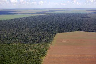
Here’s one stark example of why it matters: “Over the past 10 years, research in the Brazilian Amazon has shown that forest degradation—caused by forest fragmentation, unsustainable forestry, and fires that damaged trees—generated three times more carbon emissions than deforestation,” Bérenger said.

If you compare two similarly sized tracts of forests, the deforested tract will generate more emissions than the degraded one. But forest degradation tends to occur on a much larger scale.  

The human element

A quarter of the world’s forests are managed by people who rely on their natural resources to survive. Both deforestation and forest degradation can take a terrible toll on these communities.

That’s why the Rainforest Alliance has long collaborated with rural communities to build businesses that allow them to make a living from the forest while protecting it. The community-run concessions we partner with in Guatemala’s Maya Biosphere Reserve have done an even better job of keeping their forests healthy and intact than neighboring areas zoned for strict protection.

Europe’s pioneering new law

The Rainforest Alliance partners with farm and forest communities all over the world to protect forests. As consumers we can all do our part by buying foods, beverages, and timber items that are certified, either by the Rainforest Alliance or the Forest Stewardship Council (FSC).

But arguably, it’s companies that have the most power—and responsibility—to protect forests. The European Union is now putting the onus on big business with a new law that forces companies to eliminate deforestation and forest degradation from their supply chains.

Set to take effect in December 2024, the EU’s regulation on deforestation-free products (known as the EUDR) states that companies can only sell products in the EU, or export products made there, if they are deforestation-free and have been legally produced. The new law applies to wood, palm oil, soy, coffee, cocoa, rubber, and beef as well as most of the goods derived from these commodities. Thanks to the lobbying efforts of a coalition of NGOs, including the Rainforest Alliance, the EUDR addresses the impacts of forest degradation as well—specifically, the conversion of natural forests to tree plantations, or into a bush-type forest. The law prohibits the sale of any products originating in forests that have been transformed into plantations after December 31st, 2020.

The path forward

Until now, the terms severe degradation and deforestation have been used interchangeably, Bérenger said, but the EUDR represents the first time that an actionable definition of degradation has been sought and applied—and tied to a corresponding sanction. This landmark law paves the way for more clarity and action on forest degradation.

Ultimately, the key to keeping forests healthy and thriving lies in exactly the kind of work the Rainforest Alliance has been doing for decades. (In fact, the requirements of the EUDR closely align with the requirements of our certification program.) With more governments and companies getting on board with our vision, we’re even better equipped to create a world where people and nature thrive in harmony.

Support Our Work

May 30, 2020

Rethinking Easter Island’s Historic ‘Collapse’

Controversial new archaeological research casts doubt on a classic theory of this famous island's societal collapse

By Tom Garlinghouse & Sapiens

Daniel Frauchiger Getty Images

Easter Island’s colossal statues loom large—both literally and figuratively—in the popular imagination. The massive heads and torsos dot the landscape like stone sentinels, standing guard over the isle’s treeless, grassy expanse.

The statues have inspired widespread speculation, awe, and wonder for centuries. But the island, called Rapa Nui by its Indigenous people, has also captured the world’s imagination for an entirely different reason.

Rapa Nui is often seen as a cautionary example of societal collapse. In this story, made popular by geographer Jared Diamond’s bestselling book  Collapse , the Indigenous people of the island, the Rapanui, so destroyed their environment that, by around 1600, their society fell into a downward spiral of warfare, cannibalism, and population decline. These catastrophes, the collapse narrative explains, resulted in the destruction of the social and political structures that were in place during precolonial times, though the people of Rapa Nui survive and persist on the island to the present day.

On supporting science journalism

If you're enjoying this article, consider supporting our award-winning journalism by subscribing . By purchasing a subscription you are helping to ensure the future of impactful stories about the discoveries and ideas shaping our world today.

In recent years, researchers working on the island have  questioned this long-accepted story . For example, anthropologist Terry Hunt and archaeologist Carl Lipo, who have studied the island’s archaeology and cultural history for many years, have suggested  an alternative hypothesis  that the Rapanui did not succumb to a downward spiral of self-destruction but instead practiced resiliency, cooperation, and perhaps even a degree of environmental stewardship.

Now new evidence from Hunt, Lipo, and their colleagues,  published in the  Journal of Archaeological Science , lends credence to their ideas. This evidence suggests that the people of the island continued to thrive, as indicated by the continued construction of the stone platforms, called  ahu , on which the iconic statues stand, even after the 1600s.

“Our research shows that statue platform construction and use did not end prior to European arrival in 1722,” says Robert DiNapoli, a doctoral student in anthropology at the University of Oregon, who led the study.

This finding, drawing on new statistical methods and excavation work, suggests that the Rapanui were not destitute when the first Europeans arrived. It’s therefore possible that it was the newcomers from Europe who contributed to the island’s societal collapse in the years to come.

The new work is controversial, and not everyone is convinced. But if DiNapoli and his team are correct, the popular story of Rapa Nui’s decline, as described by Diamond, needs to be rethought and its heroes and villains reconfigured. Instead of the Rapanui hastening their own destruction prior to European contact, it is possible that the people of the island may have been the victims of European exploration and exploitation.

Rapa Nui is one of the most remote islands in the world. A tiny speck in the eastern Pacific, it sits more than 2,000 miles west of South America and is about 1,200 miles from its nearest island neighbor, Pitcairn Island.

Archaeologists have documented at least 360 ahu, most of which cluster along the island’s shoreline. They vary in configuration, though most are typically rectangular in shape and are made of basaltic stones neatly fitted together. In addition to their use as statue platforms, the ahu functioned as shrines and places of burial.

DiNapoli and his colleagues used existing radiocarbon dates from previous excavations at 11 different ahu sites. They employed what is called Bayesian analyses, which allow scientists to model the probability of specific events, to build a more precise timeline of construction activities at each site.

The new research indicates that ahu construction began soon after the first Polynesian settlers arrived on the island and continued even after European contact in 1722. This timeline argues against the hypothesized societal collapse occurring around 1600.

The downturn of the islanders, DiNapoli and his colleagues claim, began only after Europeans ushered in a period characterized by disease, murder, slave raiding, and other conflicts.

Not all Rapa Nui specialists agree with DiNapoli and his colleagues’ methods or conclusions. Jo Anne Van Tilburg, an archaeologist at the University of California, Los Angeles, is skeptical that all the radiocarbon dates used by the team reflect specifically ahu-related building events.

Van Tilburg also argues that Diamond’s environmental destruction argument remains a viable hypothesis. “The collapse narrative as these authors describe it is a straw man they have set up that does not accurately reflect the actual hypothesis,” she says.

If Europeans were to blame for the decline of Rapanui society, it would be similar to what happened to Indigenous peoples elsewhere.

In short, Van Tilburg believes the new work is missing some of the nuances of Diamond’s original theory. Diamond never described the collapse as a one-time event, Van Tilburg explains, but rather as a series of events that ultimately resulted in destructive societal changes that were hastened by European contact.

Diamond’s hypothesis is based on a mix of oral tradition, evidence of island deforestation, and the work of previous researchers, such as the Norwegian explorer and ethnologist Thor Heyerdahl. (Heyerdahl gained fame in 1947 for sailing a balsa raft, the  Kon-Tiki , to test the theory that South Americans may have colonized Polynesia.)

Early 20th-century oral historians working on Rapa Nui theorized that an internecine clash had occurred between islanders. Heyerdahl later popularized his belief that this warfare, combined with deforestation, resulted in the collapse of the island’s social hierarchies and many traditions, such as the building of stone platforms and statues.

The fate of Rapa Nui has been heatedly debated over the last several years with the development of new theories and innovative techniques, such as Bayesian methods. For many archaeologists, the pre-contact collapse theory is ripe for questioning.

Speaking of the research conducted by DiNapoli’s team, for example, Seth Quintus, an anthropologist at the University of Hawaiʻi, Mānoa, who was not involved in the study, says, “Their work adds to the growing body of evidence that has accumulated over the last 10 years that the previous narratives of collapse on Easter Island are not correct—and need to be rethought.”

If Europeans were to blame for the decline of Rapanui society, that explanation is similar to what happened to other Indigenous peoples elsewhere throughout the world, DiNapoli notes. From that perspective, he says, the popular story of environmental destruction has obscured the islanders’ successes.

“The degree to which their cultural heritage was passed on—and is still present today through language, arts, and cultural practices—is quite notable and impressive,” DiNapoli says. “This degree of resilience has been overlooked due to the collapse narrative and deserves recognition.”

This work first appeared on  SAPIENS  under a  CC BY-ND 4.0 license . Read the  original here .