hypothesis testing for single variance

school Campus Bookshelves
menu_book Bookshelves
perm_media Learning Objects
login Login
how_to_reg Request Instructor Account
hub Instructor Commons
Download Page (PDF)
Download Full Book (PDF)
Periodic Table
Physics Constants
Scientific Calculator
Reference & Cite
Tools expand_more
Readability

selected template will load here

This action is not available.

11.7: Test of a Single Variance

Last updated
Save as PDF
Page ID 1363

A test of a single variance assumes that the underlying distribution is normal . The null and alternative hypotheses are stated in terms of the population variance (or population standard deviation). The test statistic is:

\[\chi^{2} = \frac{(n-1)s^{2}}{\sigma^{2}} \label{test}\]

\(n\) is the the total number of data
\(s^{2}\) is the sample variance
\(\sigma^{2}\) is the population variance

You may think of \(s\) as the random variable in this test. The number of degrees of freedom is \(df = n - 1\). A test of a single variance may be right-tailed, left-tailed, or two-tailed. The next example will show you how to set up the null and alternative hypotheses. The null and alternative hypotheses contain statements about the population variance.

Example \(\PageIndex{1}\)

Math instructors are not only interested in how their students do on exams, on average, but how the exam scores vary. To many instructors, the variance (or standard deviation) may be more important than the average.

Suppose a math instructor believes that the standard deviation for his final exam is five points. One of his best students thinks otherwise. The student claims that the standard deviation is more than five points. If the student were to conduct a hypothesis test, what would the null and alternative hypotheses be?

Even though we are given the population standard deviation, we can set up the test using the population variance as follows.

\(H_{0}: \sigma^{2} = 5^{2}\)
\(H_{a}: \sigma^{2} > 5^{2}\)

Exercise \(\PageIndex{1}\)

A SCUBA instructor wants to record the collective depths each of his students dives during their checkout. He is interested in how the depths vary, even though everyone should have been at the same depth. He believes the standard deviation is three feet. His assistant thinks the standard deviation is less than three feet. If the instructor were to conduct a test, what would the null and alternative hypotheses be?

\(H_{0}: \sigma^{2} = 3^{2}\)
\(H_{a}: \sigma^{2} > 3^{2}\)

Example \(\PageIndex{2}\)

With individual lines at its various windows, a post office finds that the standard deviation for normally distributed waiting times for customers on Friday afternoon is 7.2 minutes. The post office experiments with a single, main waiting line and finds that for a random sample of 25 customers, the waiting times for customers have a standard deviation of 3.5 minutes.

With a significance level of 5%, test the claim that a single line causes lower variation among waiting times (shorter waiting times) for customers .

Since the claim is that a single line causes less variation, this is a test of a single variance. The parameter is the population variance, \(\sigma^{2}\), or the population standard deviation, \(\sigma\).

Random Variable: The sample standard deviation, \(s\), is the random variable. Let \(s = \text{standard deviation for the waiting times}\).

\(H_{0}: \sigma^{2} = 7.2^{2}\)
\(H_{a}: \sigma^{2} < 7.2^{2}\)

The word "less" tells you this is a left-tailed test.

Distribution for the test: \(\chi^{2}_{24}\), where:

\(n = \text{the number of customers sampled}\)
\(df = n - 1 = 25 - 1 = 24\)

Calculate the test statistic (Equation \ref{test}):

\[\chi^{2} = \frac{(n-1)s^{2}}{\sigma^{2}} = \frac{(25-1)(3.5)^{2}}{7.2^{2}} = 5.67 \nonumber\]

where \(n = 25\), \(s = 3.5\), and \(\sigma = 7.2\).

Probability statement: \(p\text{-value} = P(\chi^{2} < 5.67) = 0.000042\)

Compare \(\alpha\) and the \(p\text{-value}\) :

\[\alpha = 0.05 (p\text{-value} = 0.000042 \alpha > p\text{-value} \nonumber\]

Make a decision: Since \(\alpha > p\text{-value}\), reject \(H_{0}\). This means that you reject \(\sigma^{2} = 7.2^{2}\). In other words, you do not think the variation in waiting times is 7.2 minutes; you think the variation in waiting times is less.

Conclusion: At a 5% level of significance, from the data, there is sufficient evidence to conclude that a single line causes a lower variation among the waiting times or with a single line, the customer waiting times vary less than 7.2 minutes.

In 2nd DISTR , use 7:χ2cdf . The syntax is (lower, upper, df) for the parameter list. For Example , χ2cdf(-1E99,5.67,24) . The \(p\text{-value} = 0.000042\).

Exercise \(\PageIndex{2}\)

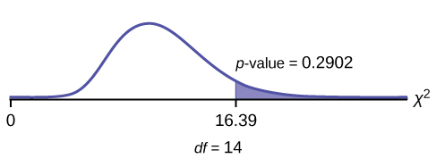
The FCC conducts broadband speed tests to measure how much data per second passes between a consumer’s computer and the internet. As of August of 2012, the standard deviation of Internet speeds across Internet Service Providers (ISPs) was 12.2 percent. Suppose a sample of 15 ISPs is taken, and the standard deviation is 13.2. An analyst claims that the standard deviation of speeds is more than what was reported. State the null and alternative hypotheses, compute the degrees of freedom, the test statistic, sketch the graph of the p -value, and draw a conclusion. Test at the 1% significance level.

\(H_{0}: \sigma^{2} = 12.2^{2}\)
\(H_{a}: \sigma^{2} > 12.2^{2}\)

In 2nd DISTR , use7: χ2cdf . The syntax is (lower, upper, df) for the parameter list. χ2cdf(16.39,10^99,14) . The \(p\text{-value} = 0.2902\).

\(df = 14\)

\[\text{chi}^{2} \text{test statistic} = 16.39 \nonumber\]

The \(p\text{-value}\) is \(0.2902\), so we decline to reject the null hypothesis. There is not enough evidence to suggest that the variance is greater than \(12.2^{2}\).

“AppleInsider Price Guides.” Apple Insider, 2013. Available online at http://appleinsider.com/mac_price_guide (accessed May 14, 2013).
Data from the World Bank, June 5, 2012.

To test variability, use the chi-square test of a single variance. The test may be left-, right-, or two-tailed, and its hypotheses are always expressed in terms of the variance (or standard deviation).

Formula Review

\(\chi^{2} = \frac{(n-1) \cdot s^{2}}{\sigma^{2}}\) Test of a single variance statistic where:

\(n: \text{sample size}\)

\(s: \text{sample standard deviation}\)

\(\sigma: \text{population standard deviation}\)

\(df = n – 1 \text{Degrees of freedom}\)

Test of a Single Variance

Use the test to determine variation.
The degrees of freedom is the \(\text{number of samples} - 1\).
The test statistic is \(\frac{(n-1) \cdot s^{2}}{\sigma^{2}}\), where \(n = \text{the total number of data}\), \(s^{2} = \text{sample variance}\), and \(\sigma^{2} = \text{population variance}\).
The test may be left-, right-, or two-tailed.

Use the following information to answer the next three exercises: An archer’s standard deviation for his hits is six (data is measured in distance from the center of the target). An observer claims the standard deviation is less.

Exercise \(\PageIndex{3}\)

What type of test should be used?

a test of a single variance

Exercise \(\PageIndex{4}\)

State the null and alternative hypotheses.

Exercise \(\PageIndex{5}\)

Is this a right-tailed, left-tailed, or two-tailed test?

a left-tailed test

Use the following information to answer the next three exercises: The standard deviation of heights for students in a school is 0.81. A random sample of 50 students is taken, and the standard deviation of heights of the sample is 0.96. A researcher in charge of the study believes the standard deviation of heights for the school is greater than 0.81.

Exercise \(\PageIndex{6}\)

\(H_{0}: \sigma^{2} = 0.81^{2}\);

\(H_{a}: \sigma^{2} > 0.81^{2}\)

\(df =\) ________

Use the following information to answer the next four exercises: The average waiting time in a doctor’s office varies. The standard deviation of waiting times in a doctor’s office is 3.4 minutes. A random sample of 30 patients in the doctor’s office has a standard deviation of waiting times of 4.1 minutes. One doctor believes the variance of waiting times is greater than originally thought.

Exercise \(\PageIndex{7}\)

Exercise \(\pageindex{8}\).

What is the test statistic?

Exercise \(\PageIndex{9}\)

What is the \(p\text{-value}\)?

Exercise \(\PageIndex{10}\)

What can you conclude at the 5% significance level?

Lecture 14: Hypothesis Test for One Variance

STAT 205: Introduction to Mathematical Statistics

University of British Columbia Okanagan

March 17, 2024

Introduction

We have covered three hypothesis tests for a single sample:

Hypothesis test for the mean \(\mu\) with \(\sigma\) known ( \(Z\) - test)
Hypothesis tests for the proportion \(p\) ( \(Z\) - test)
Hypothesis test for the mean \(\mu\) with \(\sigma\) unknown ( \(t\) -test)

Today we consider hypothesis tests involve the population variance \(\sigma^2\)

Assumptions: \(X_1, X_2, \dots, X_n\) are i.i.d + assumptions in the rhombuses.

In Lecture 7 we saw how to construct a confidence interval for \(\sigma^2\) based on the sampling distribution derived in Lecture 8 .

For random samples from normal populations , we know:

\[ \dfrac{(n-1)S^2}{\sigma^2} \sim \chi^2_{n-1} \]

where \(S^2 = \frac{\sum_{i = 1}^n (X_i - \bar{X})}{n-1}\) is the sample variance and \(\chi^2_{n-1}\) is the Chi-squared distribution with \(n-1\) degrees of freedom.

We may which to test if there is evidence to suggest that population variance differs for some hypothesized value \(\sigma_0^2\) .

As before, we start with a null hypothesis ( \(H_0\) ) that the population variance equals a specified value ( \(\sigma^2 = \sigma_0^2\) )

We test this against the alternative hypothesis \(H_A\) which can either be one-sided ( \(\sigma^2 < \sigma_0^2\) or \(\sigma^2 > \sigma_0^2\) ) or two-sided ( \(\sigma^2 \neq \sigma_0^2\) ).

Test Statistic

Recall that our test statistic is calculated assuming the null hypothesis is true . Hence, if we are testing \(H_0: \sigma^2 = \sigma_0^2\) , the test statistic we use is : \[ \chi^2 = \dfrac{(n-1)S^2}{\sigma_0^2} \] where \(\chi^2 \sim \chi^2_{n-1}\) .

Chi-square distrbituion

Assumptions

For the following inference procedures to be valid we require:

A simple random sample from the population
A normally distributed population (very important, even for large sample sizes)

It is important to note that if the population is not approximately normally distributed, chi-squared distribution may not accurately represent the sampling distribution of the test statistic.

Critical Region (upper-tailed)

The rejection region associated with an upper-tailed test for the population variance. Note that the critical value will depend on the chosen significance level ( \(\alpha\) ) and the d.f.

Critical Region (lower-tailed)

Critical Region (two-tailed)

Similarly we can find \(p\) -values from Chi-squared tables or R

\(p\) -value for lower-tailed: \[\Pr(\chi^2 < \chi^2_{\text{obs}})\] \(p\) -value for upper-tailed: \[\Pr(\chi^2 > \chi^2_{\text{obs}})\] \(p\) -value for two-tailed:

\[2\cdot \min \{ \Pr(\chi^2 < \chi^2_{\text{obs}}), \Pr(\chi^2 > \chi^2_{\text{obs}})\}\]

Exercise 1: Beyond Burger Fat

Beyond Burgers claim to have 18g grams of fat. A random sample of 6 burgers had a mean of 19.45 and a variance of 0.85 grams \(^2\) . Suppose that the quality assurance team at the company will on accept at most a \(\sigma\) of 0.5. Use the 0.05 level of significance to test the null hypotehsis \(\sigma = 0.5\) against the appropriate alternative.

Distribution of Test Statistic

Under the null hypothesis, the test statistic follows \(\chi^2 = (n-1)S^2/0.5^2\) a chi-square distribution with df = 5

Critical value

The critical value can be found by determining what value on the chi-square curve with 5 df yield a 5 percent probability in the upper tail (since we are doing an upper-tailed test). In R: qchisq(alpha, df=n-1, lower.tail = FALSE) . Verify using \(\chi^2\) table.

Observed Test Statistic

Compute the observed test statistic which we denote by \(\chi^2_{\text{obs}}\)

Since the observed test statistic falls in the rejection region, i.e. \(\chi^2_{\text{obs}} > \chi^2_{\alpha}\) , we rejection the null hypothesis in favour of the alternative.

P-value in R

Alternatively we could compute the p-value which in this case is 0.013. Since this is smaller than the alpha-level of 0.05, we reject the null hypothesis in favour of the alternative. Verify using \(\chi^2\) table.

P-value from tables

Using the chi-square distribution table we can see that our observed test statistic falls between two values. We can use the neigbouring values to approximate our p-value.

Approximate P-value

It is clear from the visualization that \[\begin{align} \Pr(\chi^2_{5} > \chi^2_{0.025}) > \Pr(\chi^2_{5} > \chi^2_{\text{obs}})\\ \Pr(\chi^2_{5} > \chi^2_{\text{obs}}) < \Pr(\chi^2_{5} > \chi^2_{0.01}) \\ \end{align}\]

The \(p\) -value, \(\Pr(\chi^2_{5} > 14.45)\) can then be expressed as: \[\begin{align} 0.01 < p\text{-value } < 0.025 \end{align}\]

the \(p\) -value (0.013) is less than \(\alpha\) = 0.05 OR
the the observed test statistic ( \(\chi^2_{\text{obs}}\) = 14.45) is larger than the critical value \(\chi^2_{\alpha}\)

we reject the null hypothesis in favour of the alternative. More specifically, there is very strong evidence to suggest that the population variance \(\sigma^2\) is greater than \(0.5^2\) .

https://irene.vrbik.ok.ubc.ca/quarto/stat205/

Module 11: The Chi Square Distribution

Hypothesis test for variance, learning outcomes.

Conduct a hypothesis test on one variance and interpret the conclusion in context

Recall: STANDARD DEVIATION AND VARIANCE

The most common measure of variation, or spread, is the standard deviation. The standard deviation is a number that measures how far data values are from their mean.

To calculate the standard deviation, we need to calculate the variance first. The variance is the average of the squares of the deviations [latex](x- \overline{x})[/latex] values for a sample, or the [latex]x – μ[/latex] values for a population). The symbol [latex]\sigma ^2[/latex] represents the population variance; the population standard deviation [latex]σ[/latex] is the square root of the population variance. The symbol [latex]s^2[/latex] represents the sample variance; the sample standard deviation [latex]s[/latex] is the square root of the sample variance.

The variance is a squared measure and does not have the same units as the data. Taking the square root solves the problem. The standard deviation measures the spread in the same units as the data.

[latex]\displaystyle\dfrac{\left(n-1\right)s^2}{\sigma^2}[/latex]

[latex]n[/latex] = the total number of data
[latex]s^2[/latex] = sample variance
[latex]\sigma^2[/latex] = population variance

You may think of [latex]s[/latex] as the random variable in this test. The number of degrees of freedom is [latex]df=n-1[/latex]. A test of a single variance may be right-tailed, left-tailed, or two-tailed. The example below will show you how to set up the null and alternative hypotheses. The null and alternative hypotheses contain statements about the population variance.

Even though we are given the population standard deviation, we can set up the test using the population variance as follows.

H 0 : σ 2 = 5 2 H a : σ 2 > 5 2

A scuba instructor wants to record the collective depths of each of his students’ dives during their checkout. He is interested in how the depths vary, even though everyone should have been at the same depth. He believes the standard deviation is three feet. His assistant thinks the standard deviation is less than three feet. If the instructor were to conduct a test, what would the null and alternative hypotheses be?

Recall: ORDER OF OPERATIONS

To calculate the test statistic follow the following steps:.

1st find the numerator:

Step 1: Calculate [latex](n-1)[/latex] by reading the problem or counting the total number of data points and then subtract [latex]1[/latex].

Step 2: Calculate [latex]s^2[/latex], and find the variance from the sample. This can be given to you in the problem or can be calculated with the following formula described in Module 2.

[latex]s^2= \frac{\sum (x- \overline{x})^2}{n-1}[/latex]. Note if you are performing a test of a single standard deviation,

Step 3: Multiply the values you got in Step 1 and Step 2.

Note: if you are performing a test of a single standard deviation, in step 2, calculate the standard deviation, [latex]s[/latex], by taking the square root of the variance.

2nd find the denominator: If you are performing a test of a single variance, read the problem or calculate the population variance with the data. If you are performing a test of a single standard deviation, read the problem or calculate the population standard deviation with the data.

Formula for the Population Variance: [latex]\sigma ^2 = \frac{\sum (x- \mu)^2}{N}[/latex]

Formula for the Population Standard Deviation: [latex]\sigma = \sqrt{\frac{\sum (x- \mu)^2}{N}}[/latex]

3rd take the numerator and divide by the denominator.

With a significance level of 5%, test the claim that a single line causes lower variation among waiting times (shorter waiting times) for customers .

Since the claim is that a single line causes less variation, this is a test of a single variance. The parameter is the population variance, σ 2 , or the population standard deviation, σ .

Random Variable: The sample standard deviation, s , is the random variable. Let s = standard deviation for the waiting times.

H 0 : σ 2 = 7.22 H a : σ 2 < 7.22

The word “less” tells you this is a left-tailed test.

Distribution for the test: [latex]X^2_{24}[/latex], where:

n = the number of customers sampled
df = n – 1 = 25 – 1 = 24

Calculate the test statistic:

X 2 = [latex]\dfrac{\left ( n-1 \right )s^2}{\sigma^2}[/latex] = [latex]\dfrac{\left ( 25-1 \right )\left ( 3.5 \right )^2}{7.2^2}[/latex] = 5.67

where n = 25, s = 3.5, and σ = 7.2.

This is a nonsymmetrical chi-square curve with values of 0 and 5.67 labeled on the horizontal axis. The point 5.67 lies to the left of the peak of the curve. A vertical upward line extends from 5.67 to the curve and the region to the left of this line is shaded. The shaded area is equal to the p-value.

Probability statement: p -value = P (χ 2 < 5.67) = 0.000042

Compare α and the p -value:

α = 0.05; p -value = 0.000042; α > p -value

Make a decision: Since α > p -value, reject H 0 . This means that you reject σ 2 = 7.22. In other words, you do not think the variation in waiting times is 7.2 minutes; you think the variation in waiting times is less.

Using a calculator:

In 2nd DISTR , use 7:χ2cdf . The syntax is (lower, upper, df) for the parameter list. For this example, χ 2 cdf(-1E99,5.67,24) . The p -value = 0.000042.

The FCC conducts broadband speed tests to measure how much data per second passes between a consumer’s computer and the internet. As of August 2012, the standard deviation of Internet speeds across Internet Service Providers (ISPs) was 12.2 percent. Suppose a sample of 15 ISPs is taken, and the standard deviation is 13.2. An analyst claims that the standard deviation of speeds is more than what was reported. State the null and alternative hypotheses, compute the degrees of freedom and the test statistic, sketch the graph of the p -value, and draw a conclusion. Test at the 1% significance level.

Introductory Statistics. Authored by : Barbara Illowsky, Susan Dean. Provided by : OpenStax. Located at : https://openstax.org/books/introductory-statistics/pages/1-introduction . License : CC BY: Attribution . License Terms : Access for free at https://openstax.org/books/introductory-statistics/pages/1-introduction

Want to create or adapt books like this? Learn more about how Pressbooks supports open publishing practices.

The Chi-Square Distribution

Test of a Single Variance

OpenStaxCollege

[latexpage]

n = the total number of data
s 2 = sample variance
σ 2 = population variance

You may think of s as the random variable in this test. The number of degrees of freedom is df = n – 1. A test of a single variance may be right-tailed, left-tailed, or two-tailed. [link] will show you how to set up the null and alternative hypotheses. The null and alternative hypotheses contain statements about the population variance.

Even though we are given the population standard deviation, we can set up the test using the population variance as follows.

H 0 : σ 2 = 5 2
H a : σ 2 > 5 2

H 0 : σ 2 = 3 2

H a : σ 2 < 3 2

With a significance level of 5%, test the claim that a single line causes lower variation among waiting times (shorter waiting times) for customers .

Since the claim is that a single line causes less variation, this is a test of a single variance. The parameter is the population variance, σ 2 , or the population standard deviation, σ .

Random Variable: The sample standard deviation, s , is the random variable. Let s = standard deviation for the waiting times.

H 0 : σ 2 = 7.2 2
H a : σ 2 < 7.2 2

The word “less” tells you this is a left-tailed test.

Distribution for the test: \({\chi }_{24}^{2}\), where:

Calculate the test statistic:

\({\chi }^{2}=\frac{\left(n\text{ }-\text{ }1\right){s}^{2}}{{\sigma }^{2}}=\frac{\left(25\text{ }-\text{ }1\right){\left(3.5\right)}^{2}}{{7.2}^{2}}=5.67\)

where n = 25, s = 3.5, and σ = 7.2.

Probability statement: p -value = P ( χ 2 < 5.67) = 0.000042

Compare α and the p -value:

α = 0.05 p -value = 0.000042 α > p -value

Make a decision: Since α > p -value, reject H 0 . This means that you reject σ 2 = 7.2 2 . In other words, you do not think the variation in waiting times is 7.2 minutes; you think the variation in waiting times is less.

In 2nd DISTR , use 7:χ2cdf . The syntax is (lower, upper, df) for the parameter list. For [link] , χ2cdf(-1E99,5.67,24) . The p -value = 0.000042.

H 0 : σ 2 = 12.2 2

H a : σ 2 > 12.2 2

chi 2 test statistic = 16.39

The p -value is 0.2902, so we decline to reject the null hypothesis. There is not enough evidence to suggest that the variance is greater than 12.2 2 .

In 2nd DISTR , use7: χ2cdf . The syntax is (lower, upper, df) for the parameter list. χ2cdf(16.39,10^99,14) . The p -value = 0.2902.

“AppleInsider Price Guides.” Apple Insider, 2013. Available online at http://appleinsider.com/mac_price_guide (accessed May 14, 2013).

Data from the World Bank, June 5, 2012.

Chapter Review

Formula Review

\({\chi }^{2}=\)\(\frac{\left(n-1\right)\cdot {s}^{2}}{{\sigma }^{2}}\) Test of a single variance statistic where:

n : sample size

s : sample standard deviation

σ : population standard deviation

df = n – 1 Degrees of freedom

Use the test to determine variation.
The degrees of freedom is the number of samples – 1.
The test statistic is \(\frac{\left(n–1\right)\cdot {s}^{2}}{{\sigma }^{2}}\), where n = the total number of data, s 2 = sample variance, and σ 2 = population variance.
The test may be left-, right-, or two-tailed.

What type of test should be used?

a test of a single variance

State the null and alternative hypotheses.

Is this a right-tailed, left-tailed, or two-tailed test?

a left-tailed test

H 0 : σ 2 = 0.81 2 ;

H a : σ 2 > 0.81 2

df = ________

What is the test statistic?

What is the p -value?

What can you conclude at the 5% significance level?

Use the following information to answer the next twelve exercises: Suppose an airline claims that its flights are consistently on time with an average delay of at most 15 minutes. It claims that the average delay is so consistent that the variance is no more than 150 minutes. Doubting the consistency part of the claim, a disgruntled traveler calculates the delays for his next 25 flights. The average delay for those 25 flights is 22 minutes with a standard deviation of 15 minutes.

Is the traveler disputing the claim about the average or about the variance?

A sample standard deviation of 15 minutes is the same as a sample variance of __________ minutes.

H 0 : __________

H 0 : σ 2 ≤ 150

chi-square test statistic = ________

p -value = ________

Graph the situation. Label and scale the horizontal axis. Mark the mean and test statistic. Shade the p -value.

Check student’s solution.

Let α = 0.05

Decision: ________

Conclusion (write out in a complete sentence.): ________

How did you know to test the variance instead of the mean?

The claim is that the variance is no more than 150 minutes.

If an additional test were done on the claim of the average delay, which distribution would you use?

If an additional test were done on the claim of the average delay, but 45 flights were surveyed, which distribution would you use?

a Student’s t – or normal distribution

For each word problem, use a solution sheet to solve the hypothesis test problem. Go to [link] for the chi-square solution sheet. Round expected frequency to two decimal places.

A plant manager is concerned her equipment may need recalibrating. It seems that the actual weight of the 15 oz. cereal boxes it fills has been fluctuating. The standard deviation should be at most 0.5 oz. In order to determine if the machine needs to be recalibrated, 84 randomly selected boxes of cereal from the next day’s production were weighed. The standard deviation of the 84 boxes was 0.54. Does the machine need to be recalibrated?

Consumers may be interested in whether the cost of a particular calculator varies from store to store. Based on surveying 43 stores, which yielded a sample mean of 💲84 and a sample standard deviation of 💲12, test the claim that the standard deviation is greater than 💲15.

H 0 : σ = 15
H a : σ > 15
chi-square with df = 42
test statistic = 26.88
p -value = 0.9663
Alpha = 0.05
Decision: Do not reject null hypothesis.

Reason for decision: p -value > alpha

Conclusion: There is insufficient evidence to conclude that the standard deviation is greater than 15.

Isabella, an accomplished Bay to Breakers runner, claims that the standard deviation for her time to run the 7.5 mile race is at most three minutes. To test her claim, Rupinder looks up five of her race times. They are 55 minutes, 61 minutes, 58 minutes, 63 minutes, and 57 minutes.

Airline companies are interested in the consistency of the number of babies on each flight, so that they have adequate safety equipment. They are also interested in the variation of the number of babies. Suppose that an airline executive believes the average number of babies on flights is six with a variance of nine at most. The airline conducts a survey. The results of the 18 flights surveyed give a sample average of 6.4 with a sample standard deviation of 3.9. Conduct a hypothesis test of the airline executive’s belief.

H 0 : σ ≤ 3
H a : σ > 3
chi-square distribution with df = 17
test statistic = 28.73
p -value = 0.0371

Alpha: 0.05

Decision: Reject the null hypothesis.
Reason for decision: p -value < alpha
Conclusion: There is sufficient evidence to conclude that the standard deviation is greater than three.

The number of births per woman in China is 1.6 down from 5.91 in 1966. This fertility rate has been attributed to the law passed in 1979 restricting births to one per woman. Suppose that a group of students studied whether or not the standard deviation of births per woman was greater than 0.75. They asked 50 women across China the number of births they had had. The results are shown in [link] . Does the students’ survey indicate that the standard deviation is greater than 0.75?

According to an avid aquarist, the average number of fish in a 20-gallon tank is 10, with a standard deviation of two. His friend, also an aquarist, does not believe that the standard deviation is two. She counts the number of fish in 15 other 20-gallon tanks. Based on the results that follow, do you think that the standard deviation is different from two? Data: 11; 10; 9; 10; 10; 11; 11; 10; 12; 9; 7; 9; 11; 10; 11

H 0 : σ = 2
H a : σ ≠ 2
chi-square distiribution with df = 14
chi-square test statistic = 5.2094
p -value = 0.0346
Decision: Reject the null hypothesis
Conclusion: There is sufficient evidence to conclude that the standard deviation is different than 2.

The manager of “Frenchies” is concerned that patrons are not consistently receiving the same amount of French fries with each order. The chef claims that the standard deviation for a ten-ounce order of fries is at most 1.5 oz., but the manager thinks that it may be higher. He randomly weighs 49 orders of fries, which yields a mean of 11 oz. and a standard deviation of two oz.

You want to buy a specific computer. A sales representative of the manufacturer claims that retail stores sell this computer at an average price of 💲1,249 with a very narrow standard deviation of 💲25. You find a website that has a price comparison for the same computer at a series of stores as follows: 💲1,299; 💲1,229.99; 💲1,193.08; 💲1,279; 💲1,224.95; 💲1,229.99; 💲1,269.95; 💲1,249. Can you argue that pricing has a larger standard deviation than claimed by the manufacturer? Use the 5% significance level. As a potential buyer, what would be the practical conclusion from your analysis?

The sample standard deviation is 💲34.29.

H 0 : σ 2 = 25 2

H a : σ 2 > 25 2

df = n – 1 = 7.

test statistic: \({x}^{2}= {x}_{7}^{2}= \frac{\left(n–1\right){s}^{2}}{{25}^{2}}= \frac{\left(8–1\right){\left(34.29\right)}^{2}}{{25}^{2}}=13.169\);

p -value: \(P\left({x}_{7}^{2}>13.169\right)=1–P\left({x}_{7}^{2} \le 13.169\right)=0.0681\)

Decision: Do not reject the null hypothesis.

Conclusion: At the 5% level, there is insufficient evidence to conclude that the variance is more than 625.

A company packages apples by weight. One of the weight grades is Class A apples. Class A apples have a mean weight of 150 g, and there is a maximum allowed weight tolerance of 5% above or below the mean for apples in the same consumer package. A batch of apples is selected to be included in a Class A apple package. Given the following apple weights of the batch, does the fruit comply with the Class A grade weight tolerance requirements. Conduct an appropriate hypothesis test.

(a) at the 5% significance level

(b) at the 1% significance level

Weights in selected apple batch (in grams): 158; 167; 149; 169; 164; 139; 154; 150; 157; 171; 152; 161; 141; 166; 172;

Lesson 12: Tests for Variances

Continuing our development of hypothesis tests for various population parameters, in this lesson, we'll focus on hypothesis tests for population variances . Specifically, we'll develop:

a hypothesis test for testing whether a single population variance \(\sigma^2\) equals a particular value
a hypothesis test for testing whether two population variances are equal

12.1 - One Variance

Yeehah again! The theoretical work for developing a hypothesis test for a population variance \(\sigma^2\) is already behind us. Recall that if you have a random sample of size n from a normal population with (unknown) mean \(\mu\) and variance \(\sigma^2\), then:

\(\chi^2=\dfrac{(n-1)S^2}{\sigma^2}\)

follows a chi-square distribution with n −1 degrees of freedom. Therefore, if we're interested in testing the null hypothesis:

\(H_0 \colon \sigma^2=\sigma^2_0\)

against any of the alternative hypotheses:

\(H_A \colon\sigma^2 \neq \sigma^2_0,\quad H_A \colon\sigma^2<\sigma^2_0,\text{ or }H_A \colon\sigma^2>\sigma^2_0\)

we can use the test statistic:

\(\chi^2=\dfrac{(n-1)S^2}{\sigma^2_0}\)

and follow the standard hypothesis testing procedures. Let's take a look at an example.

Example 12-1

A manufacturer of hard safety hats for construction workers is concerned about the mean and the variation of the forces its helmets transmits to wearers when subjected to an external force. The manufacturer has designed the helmets so that the mean force transmitted by the helmets to the workers is 800 pounds (or less) with a standard deviation to be less than 40 pounds. Tests were run on a random sample of n = 40 helmets, and the sample mean and sample standard deviation were found to be 825 pounds and 48.5 pounds, respectively.

Do the data provide sufficient evidence, at the \(\alpha = 0.05\) level, to conclude that the population standard deviation exceeds 40 pounds?

We're interested in testing the null hypothesis:

\(H_0 \colon \sigma^2=40^2=1600\)

against the alternative hypothesis:

\(H_A \colon\sigma^2>1600\)

Therefore, the value of the test statistic is:

\(\chi^2=\dfrac{(40-1)48.5^2}{40^2}=57.336\)

Is the test statistic too large for the null hypothesis to be true? Well, the critical value approach would have us finding the threshold value such that the probability of rejecting the null hypothesis if it were true, that is, of committing a Type I error, is small... 0.05, in this case. Using Minitab (or a chi-square probability table), we see that the cutoff value is 54.572:

That is, we reject the null hypothesis in favor of the alternative hypothesis if the test statistic \(\chi^2\) is greater than 54.572. It is. That is, the test statistic falls in the rejection region:

Therefore, we conclude that there is sufficient evidence, at the 0.05 level, to conclude that the population standard deviation exceeds 40.

Of course, the P -value approach yields the same conclusion. In this case, the P -value is the probablity that we would observe a chi-square(39) random variable more extreme than 57.336:

As the drawing illustrates, the P -value is 0.029 (as determined using the chi-square probability calculator in Minitab). Because \(P = 0.029 ≤ 0.05\), we reject the null hypothesis in favor of the alternative hypothesis.

Do the data provide sufficient evidence, at the \(\alpha = 0.05\) level, to conclude that the population standard deviation differs from 40 pounds?

In this case, we're interested in testing the null hypothesis:

\(H_A \colon\sigma^2 \neq 1600\)

The value of the test statistic remains the same. It is again:

Now, is the test statistic either too large or too small for the null hypothesis to be true? Well, the critical value approach would have us dividing the significance level \(\alpha = 0.05\) into 2, to get 0.025, and putting one of the halves in the left tail, and the other half in the other tail. Doing so (and using Minitab to get the cutoff values), we get that the lower cutoff value is 23.654 and the upper cutoff value is 58.120:

That is, we reject the null hypothesis in favor of the two-sided alternative hypothesis if the test statistic \(\chi^2\) is either smaller than 23.654 or greater than 58.120. It is not. That is, the test statistic does not fall in the rejection region:

Therefore, we fail to reject the null hypothesis. There is insufficient evidence, at the 0.05 level, to conclude that the population standard deviation differs from 40.

Of course, the P -value approach again yields the same conclusion. In this case, we simply double the P -value we obtained for the one-tailed test yielding a P -value of 0.058:

\(P=2\times P\left(\chi^2_{39}>57.336\right)=2\times 0.029=0.058\)

Because \(P = 0.058 > 0.05\), we fail to reject the null hypothesis in favor of the two-sided alternative hypothesis.

The above example illustrates an important fact, namely, that the conclusion for the one-sided test does not always agree with the conclusion for the two-sided test. If you have reason to believe that the parameter will differ from the null value in a particular direction, then you should conduct the one-sided test.

12.2 - Two Variances

Let's now recall the theory necessary for developing a hypothesis test for testing the equality of two population variances. Suppose \(X_1 , X_2 , \dots, X_n\) is a random sample of size n from a normal population with mean \(\mu_X\) and variance \(\sigma^2_X\). And, suppose, independent of the first sample, \(Y_1 , Y_2 , \dots, Y_m\) is another random sample of size m from a normal population with \(\mu_Y\) and variance \(\sigma^2_Y\). Recall then, in this situation, that:

\(\dfrac{(n-1)S^2_X}{\sigma^2_X} \text{ and } \dfrac{(m-1)S^2_Y}{\sigma^2_Y}\)

have independent chi-square distributions with n −1 and m −1 degrees of freedom, respectively. Therefore:

\( {\displaystyle F=\frac{\left[\frac{\color{red}\cancel {\color{black}(n-1)} \color{black}S_{X}^{2}}{\sigma_{x}^{2}} /\color{red}\cancel {\color{black}(n- 1)}\color{black}\right]}{\left[\frac{\color{red}\cancel {\color{black}(m-1)} \color{black}S_{Y}^{2}}{\sigma_{Y}^{2}} /\color{red}\cancel {\color{black}(m-1)}\color{black}\right]}=\frac{S_{X}^{2}}{S_{Y}^{2}} \cdot \frac{\sigma_{Y}^{2}}{\sigma_{X}^{2}}} \)

follows an F distribution with n −1 numerator degrees of freedom and m −1 denominator degrees of freedom. Therefore, if we're interested in testing the null hypothesis:

\(H_0 \colon \sigma^2_X=\sigma^2_Y\) (or equivalently \(H_0 \colon\dfrac{\sigma^2_Y}{\sigma^2_X}=1\))

\(H_A \colon \sigma^2_X \neq \sigma^2_Y,\quad H_A \colon \sigma^2_X >\sigma^2_Y,\text{ or }H_A \colon \sigma^2_X <\sigma^2_Y\)

\(F=\dfrac{S^2_X}{S^2_Y}\)

and follow the standard hypothesis testing procedures. When doing so, we might also want to recall this important fact about the F -distribution:

\(F_{1-(\alpha/2)}(n-1,m-1)=\dfrac{1}{F_{\alpha/2}(m-1,n-1)}\)

so that when we use the critical value approach for a two-sided alternative:

\(H_A \colon\sigma^2_X \neq \sigma^2_Y\)

we reject if the test statistic F is too large:

\(F \geq F_{\alpha/2}(n-1,m-1)\)

or if the test statistic F is too small:

\(F \leq F_{1-(\alpha/2)}(n-1,m-1)=\dfrac{1}{F_{\alpha/2}(m-1,n-1)}\)

Okay, let's take a look at an example. In the last lesson, we performed a two-sample t -test (as well as Welch's test) to test whether the mean fastest speed driven by the population of male college students differs from the mean fastest speed driven by the population of female college students. When we performed the two-sample t -test, we just assumed the population variances were equal. Let's revisit that example again to see if our assumption of equal variances is valid.

Example 12-2

A psychologist was interested in exploring whether or not male and female college students have different driving behaviors. The particular statistical question she framed was as follows:

Is the mean fastest speed driven by male college students different than the mean fastest speed driven by female college students?

The psychologist conducted a survey of a random \(n = 34\) male college students and a random \(m = 29\) female college students. Here is a descriptive summary of the results of her survey:

Is there sufficient evidence at the \(\alpha = 0.05\) level to conclude that the variance of the fastest speed driven by male college students differs from the variance of the fastest speed driven by female college students?

\(H_0 \colon \sigma^2_X=\sigma^2_Y\)

The value of the test statistic is:

\(F=\dfrac{12.2^2}{20.1^2}=0.368\)

(Note that I intentionally put the variance of what we're calling the Y sample in the numerator and the variance of what we're calling the X sample in the denominator. I did this only so that my results match the Minitab output we'll obtain on the next page. In doing so, we just need to make sure that we keep track of the correct numerator and denominator degrees of freedom.) Using the critical value approach , we divide the significance level \(\alpha = 0.05\) into 2, to get 0.025, and put one of the halves in the left tail, and the other half in the other tail. Doing so, we get that the lower cutoff value is 0.478 and the upper cutoff value is 2.0441:

Because the test statistic falls in the rejection region, that is, because \(F = 0.368 ≤ 0.478\), we reject the null hypothesis in favor of the alternative hypothesis. There is sufficient evidence at the \(\alpha = 0.05\) level to conclude that the population variances are not equal. Therefore, the assumption of equal variances that we made when performing the two-sample t -test on these data in the previous lesson does not appear to be valid. It would behoove us to use Welch's t -test instead.

12.3 - Using Minitab

In each case, we'll illustrate how to perform the hypothesis tests of this lesson using summarized data.

Hypothesis Test for One Variance

Under the Stat menu, select Basic Statistics , and then select 1 Variance... :

In the pop-up window that appears, in the box labeled Data , select Sample standard deviation (or alternatively Sample variance ). In the box labeled Sample size , type in the size n of the sample. In the box labeled Sample standard deviation , type in the sample standard deviation. Click on the box labeled Perform hypothesis test , and in the box labeled Value , type in the Hypothesized standard deviation (or alternatively the Hypothesized variance ):

Click on the button labeled Options... In the pop-up window that appears, for the box labeled Alternative , select either less than , greater than , or not equal depending on the direction of the alternative hypothesis:

Then, click on OK to return to the main pop-up window.

Then, upon clicking OK on the main pop-up window, the output should appear in the Session window:

Hypothesis Test for Two Variances

Under the Stat menu, select Basic Statistics , and then select 2 Variances... :

In the pop-up window that appears, in the box labeled Data , select Sample standard deviations (or alternatively Sample variances ). In the box labeled Sample size , type in the size n of the First sample and m of the Second sample. In the box labeled Standard deviation , type in the sample standard deviations for the First and Second samples:

Click on the button labeled Options... In the pop-up window that appears, in the box labeled Value , type in the Hypothesized ratio of the standard deviations (or the Hypothesized ratio of the variances ). For the box labeled Alternative , select either less than , greater than , or not equal depending on the direction of the alternative hypothesis:

Test and CI for Two Variances

Null hypothesis Sigma(1) / Sigma(2) = 1 Alternative hypothesis Sigma(1) / Sigma(2) not = 1 Significance level Alpha = 0.05

Ratio of standard deviations = 0.607 Ratio of variances = 0.368

95% Confidence Intervals

Hypothesis tests about the variance

by Marco Taboga , PhD

This page explains how to perform hypothesis tests about the variance of a normal distribution, called Chi-square tests.

We analyze two different situations:

when the mean of the distribution is known;

when it is unknown.

Depending on the situation, the Chi-square statistic used in the test has a different distribution.

At the end of the page, we propose some solved exercises.

Table of contents

Normal distribution with known mean

The null hypothesis, the test statistic, the critical region, the decision, the power function, the size of the test, how to choose the critical value, normal distribution with unknown mean, solved exercises.

The assumptions are the same previously made in the lecture on confidence intervals for the variance .

The sample is drawn from a normal distribution .

A test of hypothesis based on it is called a Chi-square test .

Otherwise the null is not rejected.

We explain how to do this in the page on critical values .

We now relax the assumption that the mean of the distribution is known.

See the comments on the choice of the critical value made for the case of known mean.

Below you can find some exercises with explained solutions.

Suppose that we observe 40 independent realizations of a normal random variable.

we run a Chi-square test of the null hypothesis that the variance is equal to 1;

Make the same assumptions of Exercise 1 above.

If the unadjusted sample variance is equal to 0.9, is the null hypothesis rejected?

How to cite

Please cite as:

Taboga, Marco (2021). "Hypothesis tests about the variance", Lectures on probability theory and mathematical statistics. Kindle Direct Publishing. Online appendix. https://www.statlect.com/fundamentals-of-statistics/hypothesis-testing-variance.

Most of the learning materials found on this website are now available in a traditional textbook format.

Convergence in probability
Multivariate normal distribution
Characteristic function
Moment generating function
Chi-square distribution
Beta function
Bernoulli distribution
Mathematical tools
Fundamentals of probability
Probability distributions
Asymptotic theory
Fundamentals of statistics
About Statlect
Cookies, privacy and terms of use
Posterior probability
IID sequence
Probability space
Probability density function
Continuous mapping theorem
To enhance your privacy,
we removed the social buttons,
but don't forget to share .

11.2 Test of a Single Variance

Thus far our interest has been exclusively on the population parameter μ or it's counterpart in the binomial, p. Surely the mean of a population is the most critical piece of information to have, but in some cases we are interested in the variability of the outcomes of some distribution. In almost all production processes quality is measured not only by how closely the machine matches the target, but also the variability of the process. If one were filling bags with potato chips not only would there be interest in the average weight of the bag, but also how much variation there was in the weights. No one wants to be assured that the average weight is accurate when their bag has no chips. Electricity voltage may meet some average level, but great variability, spikes, can cause serious damage to electrical machines, especially computers. I would not only like to have a high mean grade in my classes, but also low variation about this mean. In short, statistical tests concerning the variance of a distribution have great value and many applications.

A test of a single variance assumes that the underlying distribution is normal . The null and alternative hypotheses are stated in terms of the population variance . The test statistic is:

n = the total number of observations in the sample data
s 2 = sample variance
σ 0 2 σ 0 2 = hypothesized value of the population variance
H 0 : σ 2 = σ 0 2 H 0 : σ 2 = σ 0 2
H a : σ 2 ≠ σ 0 2 H a : σ 2 ≠ σ 0 2

You may think of s as the random variable in this test. The number of degrees of freedom is df = n - 1. A test of a single variance may be right-tailed, left-tailed, or two-tailed. Example 11.1 will show you how to set up the null and alternative hypotheses. The null and alternative hypotheses contain statements about the population variance.

Example 11.1

Even though we are given the population standard deviation, we can set up the test using the population variance as follows.

H 0 : σ 2 ≤ 5 2
H a : σ 2 > 5 2

Try It 11.1

A SCUBA instructor wants to record the collective depths each of his students' dives during their checkout. He is interested in how the depths vary, even though everyone should have been at the same depth. He believes the standard deviation is three feet. His assistant thinks the standard deviation is less than three feet. If the instructor were to conduct a test, what would the null and alternative hypotheses be?

Example 11.2

With individual lines at its various windows, a post office finds that the standard deviation for waiting times for customers on Friday afternoon is 7.2 minutes. The post office experiments with a single, main waiting line and finds that for a random sample of 25 customers, the waiting times for customers have a standard deviation of 3.5 minutes on a Friday afternoon.

With a significance level of 5%, test the claim that a single line causes lower variation among waiting times for customers .

Since the claim is that a single line causes less variation, this is a test of a single variance. The parameter is the population variance, σ 2 .

Random Variable: The sample standard deviation, s , is the random variable. Let s = standard deviation for the waiting times.

H 0 : σ 2 ≥ 7.2 2
H a : σ 2 < 7.2 2

The word "less" tells you this is a left-tailed test.

Distribution for the test: χ 24 2 χ 24 2 , where:

n = the number of customers sampled
df = n – 1 = 25 – 1 = 24

Calculate the test statistic:

χ c 2 = ( n − 1 ) s 2 σ 2 = ( 25 − 1 ) ( 3.5 ) 2 7.2 2 = 5.67 χ c 2 = ( n − 1 ) s 2 σ 2 = ( 25 − 1 ) ( 3.5 ) 2 7.2 2 = 5.67

where n = 25, s = 3.5, and σ = 7.2.

The graph of the Chi-square shows the distribution and marks the critical value with 24 degrees of freedom at 95% level of confidence, α = 0.05, 13.85. The critical value of 13.85 came from the Chi squared table which is read very much like the students t table. The difference is that the students t -distribution is symmetrical and the Chi squared distribution is not. At the top of the Chi squared table we see not only the familiar 0.05, 0.10, etc. but also 0.95, 0.975, etc. These are the columns used to find the left hand critical value. The graph also marks the calculated χ 2 test statistic of 5.67. Comparing the test statistic with the critical value, as we have done with all other hypothesis tests, we reach the conclusion.

Make a decision: Because the calculated test statistic is in the tail we cannot accept H 0 . This means that you reject σ 2 ≥ 7.2 2 . In other words, you do not think the variation in waiting times is 7.2 minutes or more; you think the variation in waiting times is less.

Example 11.3

Professor Hadley has a weakness for cream filled donuts, but he believes that some bakeries are not properly filling the donuts. A sample of 24 donuts reveals a mean amount of filling equal to 0.04 cups, and the sample standard deviation is 0.11 cups. Professor Hadley has an interest in the average quantity of filling, of course, but he is particularly distressed if one donut is radically different from another. Professor Hadley does not like surprises.

Test at 95% the null hypothesis that the population variance of donut filling is significantly different from the average amount of filling.

This is clearly a problem dealing with variances. In this case we are testing a single sample rather than comparing two samples from different populations. The null and alternative hypotheses are thus:

The test is set up as a two-tailed test because Professor Hadley has shown concern with too much variation in filling as well as too little: his dislike of a surprise is any level of filling outside the expected average of 0.04 cups. The test statistic is calculated to be:

The calculated χ 2 χ 2 test statistic, 6.96, is in the tail therefore at a 0.05 level of significance, we cannot accept the null hypothesis that the variance in the donut filling is equal to 0.04 cups. It seems that Professor Hadley is destined to meet disappointment with each bit.

Try It 11.3

The FCC conducts broadband speed tests to measure how much data per second passes between a consumer’s computer and the internet. As of August of 2012, the standard deviation of Internet speeds across Internet Service Providers (ISPs) was 12.2 percent. Suppose a sample of 15 ISPs is taken, and the standard deviation is 13.2. An analyst claims that the standard deviation of speeds is more than what was reported. State the null and alternative hypotheses, compute the degrees of freedom, the test statistic, sketch the graph of the distribution and mark the area associated with the level of confidence, and draw a conclusion. Test at the 1% significance level.

As an Amazon Associate we earn from qualifying purchases.

This book may not be used in the training of large language models or otherwise be ingested into large language models or generative AI offerings without OpenStax's permission.

Want to cite, share, or modify this book? This book uses the Creative Commons Attribution License and you must attribute OpenStax.

Access for free at https://openstax.org/books/introductory-business-statistics/pages/1-introduction

Authors: Alexander Holmes, Barbara Illowsky, Susan Dean
Publisher/website: OpenStax
Book title: Introductory Business Statistics
Publication date: Nov 29, 2017
Location: Houston, Texas
Book URL: https://openstax.org/books/introductory-business-statistics/pages/1-introduction
Section URL: https://openstax.org/books/introductory-business-statistics/pages/11-2-test-of-a-single-variance

© Jun 23, 2022 OpenStax. Textbook content produced by OpenStax is licensed under a Creative Commons Attribution License . The OpenStax name, OpenStax logo, OpenStax book covers, OpenStax CNX name, and OpenStax CNX logo are not subject to the Creative Commons license and may not be reproduced without the prior and express written consent of Rice University.

Want to create or adapt books like this? Learn more about how Pressbooks supports open publishing practices.

10.3 Statistical Inference for a Single Population Variance

Learning objectives.

Calculate and interpret a confidence interval for a population variance.
Conduct and interpret a hypothesis test on a single population variance.

The mean of a population is important, but in many cases the variance of the population is just as important. In most production processes, quality is measured by how closely the process matches the target (i.e. the mean) and by the variability (i.e. the variance) of the process. For example, if a process is to fill bags of coffee beans, we are interested in both the average weight of the bag and how much variation there is in the weight of the bags. The quality is considered poor if the average weight of the bags is accurate but the variance of the weight of the bags is too high—a variance that is too large means some bags would be too full and some bags would be almost empty.

As with other population parameters, we can construct a confidence interval to capture the population variance and conduct a hypothesis test on the population variance. In order to construct a confidence interval or conduct a hypothesis test on a population variance [latex]\sigma^2[/latex], we need to use the distribution of [latex]\displaystyle{\frac{(n-1) \times s^2}{\sigma^2}}[/latex]. Suppose we have a normal population with population variance [latex]\sigma^2[/latex] and a sample of size [latex]n[/latex] is taken from the population. The sampling distribution of [latex]\displaystyle{\frac{(n-1) \times s^2}{\sigma^2}}[/latex] follows a [latex]\chi^2[/latex]-distribution with [latex]n-1[/latex] degrees of freedom.

Constructing a Confidence Interval for a Population Variance

To construct the confidence interval, take a random sample of size [latex]n[/latex] from a normally distributed population. Calculate the sample variance [latex]s^2[/latex]. The limits for the confidence interval with confidence level [latex]C[/latex] for an unknown population variance [latex]\sigma^2[/latex] are

[latex]\begin{eqnarray*} \mbox{Lower Limit} & = & \frac{(n-1) \times s^2}{\chi^2_R} \\ \\ \mbox{Upper Limit} & = & \frac{(n-1) \times s^2}{\chi^2_L} \\ \\ \end{eqnarray*}[/latex]

where [latex]\chi^2_L[/latex] is the [latex]\chi^2[/latex]-score so that the area in the left-tail of the [latex]\chi^2[/latex]-distribution is [latex]\displaystyle{\frac{1-C}{2}}[/latex], [latex]\chi^2_R[/latex] is the [latex]\chi^2[/latex]-score so that the area in the right-tail of the [latex]\chi^2[/latex]-distribution is [latex]\displaystyle{\frac{1-C}{2}}[/latex] and the [latex]\chi^2[/latex]-distribution has [latex]n-1[/latex] degrees of freedom.

This is a chi square distribution. Along the horizontal axis the points chi square L and chi square R are labeled. The area under the curve in between chi square L and chi square R equals C%. The area in the right tail to the right of chi square R equals (1-C)/2. The area in the left tail to the left of chi square L equals (1-C)/2.

Like the other confidence intervals we have seen, the [latex]\chi^2[/latex]-scores are the values that trap [latex]C\%[/latex] of the observations in the middle of the distribution so that the area of each tail is [latex]\displaystyle{\frac{1-C}{2}}[/latex].
Because the [latex]\chi^2[/latex]-distribution is not symmetrical, the confidence interval for a population variance requires that we calculate two different [latex]\chi^2[/latex]-scores: one for the left tail and one for the right tail. In Excel, we will need to use both the chisq.inv function (for the left tail) and the chisq.inv.rt function (for the right tail) to find the two different [latex]\chi^2[/latex]-scores.
The [latex]\chi^2[/latex]-score for the left tail is part of the formula for the upper limit and the [latex]\chi^2[/latex]-score for the right tail is part of the formula for the lower limit. This is not a mistake . It follows from the formula used to determine the limits for the confidence interval.

A local telecom company conducts broadband speed tests to measure how much data per second passes between a customer’s computer and the internet compared to what the customer pays for as part of their plan . The company needs to estimate the variance in the broadband speed. A sample of 15 ISPs is taken and amount of data per second is recorded. The variance in the sample is 174.

Construct a 97% confidence interval for the variance in the amount of data per second that passes between a customer’s computer and the internet.
Interpret the confidence interval found in part 1.

This is a chi square distribution. Along the horizontal axis the point chi square L is labeled. The area in the left tail to the left of chi square L equals 1.5%

We also need find the [latex]\chi^2_R[/latex]-score for the 97% confidence interval. This means that we need to find the [latex]\chi^2_R[/latex]-score so that the area in the right tail is [latex]\displaystyle{\frac{1-0.97}{2}=0.015}[/latex]. The degrees of freedom for the [latex]\chi^2[/latex]-distribution is [latex]n-1=15-1=14[/latex].

This is a chi square distribution. Along the horizontal axis the point chi square R is labeled. The area in the left tail to the left of chi square R equals 1.5%

So [latex]\chi^2_L=5.0572...[/latex] and [latex]\chi^2_R=27.826...[/latex]. From the sample data supplied in the question [latex]s^2=174[/latex] and [latex]n=15[/latex]. The 97% confidence interval is

[latex]\begin{eqnarray*} \mbox{Lower Limit} & = & \frac{(n-1) \times s^2}{\chi^2_R} \\ & = & \frac{(15-1) \times 174}{27.826...} \\ & = & 87.54 \\ \\ \mbox{Upper Limit} & = & \frac{(n-1) \times s^2}{\chi^2_R} \\ & = & \frac{(15-1) \times 174}{5.0572...} \\ & = & 481.69 \\ \\ \end{eqnarray*}[/latex]

We are 97% confident that the variance in the amount of data per second that passes between a customer’s computer and the internet is between 87.54 and 481.69.
When calculating the limits for the confidence interval keep all of the decimals in the [latex]\chi^2[/latex]-scores and other values throughout the calculation. This will ensure that there is no round-off error in the answer. You can use Excel to do the calculations of the limits, clicking on the cells containing the [latex]\chi^2[/latex]-scores and any other values.
When writing down the interpretation of the confidence interval, make sure to include the confidence level and the actual population variance captured by the confidence interval (i.e. be specific to the context of the question). In this case, there are no units for the limits because variance does not have any limits.

Steps to Conduct a Hypothesis Test for a Population Variance

Write down the null and alternative hypotheses in terms of the population variance [latex]\sigma^2[/latex].
Use the form of the alternative hypothesis to determine if the test is left-tailed, right-tailed, or two-tailed.
Collect the sample information for the test and identify the significance level [latex]\alpha[/latex].

[latex]\begin{eqnarray*}\chi^2=\frac{(n-1) \times s^2}{\sigma^2} & \; \; \; \; \; \; \; \; & df=n-1 \\ \\ \end{eqnarray*}[/latex]

The results of the sample data are significant. There is sufficient evidence to conclude that the null hypothesis [latex]H_0[/latex] is an incorrect belief and that the alternative hypothesis [latex]H_a[/latex] is most likely correct.
The results of the sample data are not significant. There is not sufficient evidence to conclude that the alternative hypothesis [latex]H_a[/latex] may be correct.
Write down a concluding sentence specific to the context of the question.

A statistics instructor at a local college claims that the variance for the final exam scores was 25. After speaking with his classmates, one the class’s best students thinks that the variance for the final exam scores is higher than the instructor claims. The student challenges the instructor to prove her claim. The instructor takes a sample 30 final exams and finds the variance of the scores is 28. At the 5% significance level, test if the variance of the final exam scores is higher than the instructor claims.

Hypotheses:

[latex]\begin{eqnarray*} H_0: & & \sigma^2=25 \\ H_a: & & \sigma^2 \gt 25 \end{eqnarray*}[/latex]

From the question, we have [latex]n=30[/latex], [latex]s^2=28[/latex], and [latex]\alpha=0.05[/latex].

Because the alternative hypothesis is a [latex]\gt[/latex], the p -value is the area in the right tail of the [latex]\chi^2[/latex]-distribution.

This is a chi square distribution. Along the horizontal axis the point chi square is labeled. The area in the right tail to the right of chi square is shaded and labeled with p-value.

To use the chisq.dist.rt function, we need to calculate out the [latex]\chi^2[/latex]-score and the degrees of freedom:

[latex]\begin{eqnarray*} \chi^2 & = &\frac{(n-1) \times s^2}{\sigma^2} \\ & = & \frac{(30-1) \times 28}{25} \\ & = & 32.48 \\ \\ df & = & n-1 \\ & = & 30-1 \\ & = & 29 \end{eqnarray*}[/latex]

So the p -value[latex]=0.2992[/latex].

Conclusion:

Because p -value[latex]=0.2992 \gt 0.05=\alpha[/latex], we do not reject the null hypothesis. At the 5% significance level there is not enough evidence to suggest that the variance of the final exam scores is higher than 25.

The null hypothesis [latex]\sigma^2=25[/latex] is the claim that the variance on the final exam is 25.
The alternative hypothesis [latex]\sigma^2 \gt 25[/latex] is the claim that the variance on the final exam is greater than 25.
There are no units included with the hypotheses because variance does not have any units.
The function is chisq.dist.rt because we are finding the area in the right tail of a [latex]\chi^2[/latex]-distribution.
Field 1 is the value of [latex]\chi^2[/latex].
Field 2 is the degrees of freedom.
The p -value of 0.2992 is a large probability compared to the significance level, and so is likely to happen assuming the null hypothesis is true. This suggests that the assumption that the null hypothesis is true is most likely correct, and so the conclusion of the test is to not reject the null hypothesis. In other words, the variance of the scores on the final exam is most likely 25.

With individual lines at its various windows, a post office finds that the standard deviation for normally distributed waiting times for customers is 7.2 minutes. The post office experiments with a single, main waiting line and finds that for a random sample of 25 customers the waiting times for customers have a standard deviation of 4.5 minutes. At the 5% significance level, determine if the single line changed the variation among the wait times for customers.

[latex]\begin{eqnarray*} H_0: & & \sigma^2=51.84 \\ H_a: & & \sigma^2 \neq 51.84 \end{eqnarray*}[/latex]

From the question, we have [latex]n=25[/latex], [latex]s^2=20.25[/latex], and [latex]\alpha=0.05[/latex].

Because the alternative hypothesis is a [latex]\neq[/latex], the p -value is the sum of the areas in the tails of the [latex]\chi^2[/latex]-distribution.

This is a chi square distribution curve. The points chi square L and chi square R are on the horizontal axis. A vertical line extends from point chi square R to the curve with the area to the right of this vertical line shaded and labeled as one half of the p-value. A vertical line extends from chi square L to the curve with the area to the left of this vertical line shaded and labeled as one half of the p-value. The p-value equals the sum of area of these two shaded regions.

We need to calculate out the [latex]\chi^2[/latex]-score and the degrees of freedom:

[latex]\begin{eqnarray*} \chi^2 & = &\frac{(n-1) \times s^2}{\sigma^2} \\ & = & \frac{(25-1) \times 20.25}{51.84} \\ & = & 9.375 \\ \\ df & = & n-1 \\ & = & 25-1 \\ & = & 24 \end{eqnarray*}[/latex]

Because this is a two-tailed test, we need to know which tail (left or right) we have the [latex]\chi^2[/latex]-score for so that we can use the correct Excel function. If [latex]\chi^2 \gt df-2[/latex], the [latex]\chi^2[/latex]-score corresponds to the right tail. If the [latex]\chi^2 \lt df-2[/latex], the [latex]\chi^2[/latex]-score corresponds to the left tail. In this case, [latex]\chi^2=9.375 \lt 22=df-2[/latex], so the [latex]\chi^2[/latex]-score corresponds to the left tail. We need to use chisq.dist to find the area in the left tail.

So the area in the left tail is 0.0033, which means that [latex]\frac{1}{2}[/latex]( p -value)=0.0033. This is also the area in the right tail, so

p -value=[latex]0.0033+0.0033=0.0066[/latex]

Because p -value[latex]=0.0066 \lt 0.05=\alpha[/latex], we reject the null hypothesis in favour of the alternative hypothesis. At the 5% significance level there is enough evidence to suggest that the variation among the wait times for customers has changed.

The null hypothesis [latex]\sigma^2=51.84[/latex] is the claim that the variance in the wait times is 51.84. Note that we were given the standard deviation ([latex]\sigma=7.2[/latex]) in the question. But this is a test on variance, so we must write the hypotheses in terms of the variance [latex]\sigma^2=7.2^2=51.84[/latex].
The alternative hypothesis [latex]\sigma^2 \neq 51.84[/latex] is the claim that the variance in the wait times has changed from 51.84.
We use chisq.dist to find the area in the left tail. The area in the right tail equals the area in the left tail, so we can find the p -value by adding the output from this function to itself.
We use chisq.dist.rt to find the area in the right tail. The area in the left tail equals the area in the right tail, so we can find the p -value by adding the output from this function to itself.
The p -value of 0.0066 is a small probability compared to the significance level, and so is unlikely to happen assuming the null hypothesis is true. This suggests that the assumption that the null hypothesis is true is most likely incorrect, and so the conclusion of the test is to reject the null hypothesis in favour of the alternative hypothesis. In other words, the variance in the wait times has most likely changed.

A scuba instructor wants to record the collective depths each of his students dives during their checkout. He is interested in how the depths vary, even though everyone should have been at the same depth. He believes the standard deviation of the depths is 1.2 meters. But his assistant thinks the standard deviation is less than 1.2 meters. The instructor wants to test this claim. The scuba instructor uses his most recent class of 20 students as a sample and finds that the standard deviation of the depths is 0.85 meters. At the 1% significance level, test if the variability in the depths of the student scuba divers is less than claimed.

[latex]\begin{eqnarray*} H_0: & & \sigma^2=1.44 \\ H_a: & & \sigma^2 \lt 1.44 \end{eqnarray*}[/latex]

From the question, we have [latex]n=20[/latex], [latex]s^2=0.7225[/latex], and [latex]\alpha=0.01[/latex].

Because the alternative hypothesis is a [latex]\lt[/latex], the p -value is the area in the left tail of the [latex]\chi^2[/latex]-distribution.

This is a chi square distribution curve. The point chi square is on the horizontal axis. A vertical line extends from chi square to the curve with the area to the left of this vertical line shaded and labeled as the p-value.

To use the chisq.dist function, we need to calculate out the [latex]\chi^2[/latex]-score and the degrees of freedom:

[latex]\begin{eqnarray*} \chi^2 & = &\frac{(n-1) \times s^2}{\sigma^2} \\ & = & \frac{(20-1) \times 0.7225}{1.44} \\ & = & 9.5329... \\ \\ df & = & n-1 \\ & = & 20-1 \\ & = & 19 \end{eqnarray*}[/latex]

So the p -value[latex]=0.0365[/latex].

Because p -value[latex]=0.0365 \gt 0.01=\alpha[/latex], we do not reject the null hypothesis. At the 1% significance level there is not enough evidence to suggest that the variation in the depths of the students is less than claimed.

Watch this video: Hypothesis Tests for One Population Variance by jbstatistics [8:51]

Concept Review

To construct a confidence interval or conduct a hypothesis test on a population variance, we use the sampling distribution of [latex]\displaystyle{\frac{(n-1) \times s^2}{\sigma^2}}[/latex], which follows a [latex]\chi^2[/latex]-distribution with [latex]n-1[/latex] degrees of freedom.

The hypothesis test for a population variance is a well established process:

Collect the sample information for the test and identify the significance level.
Find the p -value (the area in the corresponding tail) for the test using the [latex]\chi^2[/latex]-distribution where [latex]\displaystyle{\chi^2=\frac{(n-1) \times s^2}{\sigma^2}}[/latex] and [latex]df=n-1[/latex].
Compare the p -value to the significance level and state the outcome of the test.

[latex]\begin{eqnarray*} \mbox{Lower Limit} & = & \frac{(n-1) \times s^2}{\chi^2_R} \\ \\ \mbox{Upper Limit} & = & \frac{(n-1) \times s^2}{\chi^2_L} \end{eqnarray*}[/latex]

where [latex]\chi^2_L[/latex] is the [latex]\chi^2[/latex]-score so that the area in the left-tail of of the [latex]\chi^2[/latex]-distribution is [latex]\displaystyle{\frac{1-C}{2}}[/latex], [latex]\chi^2_R[/latex] is the [latex]\chi^2[/latex]-score so that the area in the right-tail of of the [latex]\chi^2[/latex]-distribution is [latex]\displaystyle{\frac{1-C}{2}}[/latex] and the [latex]\chi^2[/latex]-distribution has [latex]n-1[/latex] degrees of freedom.

Attribution

“ 11.6 Test of a Single Variance “ in Introductory Statistics by OpenStax is licensed under a Creative Commons Attribution 4.0 International License.

Hypothesis Testing - Analysis of Variance (ANOVA)

Lisa Sullivan, PhD

Professor of Biostatistics

Boston University School of Public Health

Introduction

This module will continue the discussion of hypothesis testing, where a specific statement or hypothesis is generated about a population parameter, and sample statistics are used to assess the likelihood that the hypothesis is true. The hypothesis is based on available information and the investigator's belief about the population parameters. The specific test considered here is called analysis of variance (ANOVA) and is a test of hypothesis that is appropriate to compare means of a continuous variable in two or more independent comparison groups. For example, in some clinical trials there are more than two comparison groups. In a clinical trial to evaluate a new medication for asthma, investigators might compare an experimental medication to a placebo and to a standard treatment (i.e., a medication currently being used). In an observational study such as the Framingham Heart Study, it might be of interest to compare mean blood pressure or mean cholesterol levels in persons who are underweight, normal weight, overweight and obese.

The technique to test for a difference in more than two independent means is an extension of the two independent samples procedure discussed previously which applies when there are exactly two independent comparison groups. The ANOVA technique applies when there are two or more than two independent groups. The ANOVA procedure is used to compare the means of the comparison groups and is conducted using the same five step approach used in the scenarios discussed in previous sections. Because there are more than two groups, however, the computation of the test statistic is more involved. The test statistic must take into account the sample sizes, sample means and sample standard deviations in each of the comparison groups.

If one is examining the means observed among, say three groups, it might be tempting to perform three separate group to group comparisons, but this approach is incorrect because each of these comparisons fails to take into account the total data, and it increases the likelihood of incorrectly concluding that there are statistically significate differences, since each comparison adds to the probability of a type I error. Analysis of variance avoids these problemss by asking a more global question, i.e., whether there are significant differences among the groups, without addressing differences between any two groups in particular (although there are additional tests that can do this if the analysis of variance indicates that there are differences among the groups).

The fundamental strategy of ANOVA is to systematically examine variability within groups being compared and also examine variability among the groups being compared.

Learning Objectives

After completing this module, the student will be able to:

Perform analysis of variance by hand
Appropriately interpret results of analysis of variance tests
Distinguish between one and two factor analysis of variance tests
Identify the appropriate hypothesis testing procedure based on type of outcome variable and number of samples

The ANOVA Approach

Consider an example with four independent groups and a continuous outcome measure. The independent groups might be defined by a particular characteristic of the participants such as BMI (e.g., underweight, normal weight, overweight, obese) or by the investigator (e.g., randomizing participants to one of four competing treatments, call them A, B, C and D). Suppose that the outcome is systolic blood pressure, and we wish to test whether there is a statistically significant difference in mean systolic blood pressures among the four groups. The sample data are organized as follows:

The hypotheses of interest in an ANOVA are as follows:

H 0 : μ 1 = μ 2 = μ 3 ... = μ k
H 1 : Means are not all equal.

where k = the number of independent comparison groups.

In this example, the hypotheses are:

H 0 : μ 1 = μ 2 = μ 3 = μ 4
H 1 : The means are not all equal.

The null hypothesis in ANOVA is always that there is no difference in means. The research or alternative hypothesis is always that the means are not all equal and is usually written in words rather than in mathematical symbols. The research hypothesis captures any difference in means and includes, for example, the situation where all four means are unequal, where one is different from the other three, where two are different, and so on. The alternative hypothesis, as shown above, capture all possible situations other than equality of all means specified in the null hypothesis.

Test Statistic for ANOVA

The test statistic for testing H 0 : μ 1 = μ 2 = ... = μ k is:

and the critical value is found in a table of probability values for the F distribution with (degrees of freedom) df 1 = k-1, df 2 =N-k. The table can be found in "Other Resources" on the left side of the pages.

NOTE: The test statistic F assumes equal variability in the k populations (i.e., the population variances are equal, or s 1 2 = s 2 2 = ... = s k 2 ). This means that the outcome is equally variable in each of the comparison populations. This assumption is the same as that assumed for appropriate use of the test statistic to test equality of two independent means. It is possible to assess the likelihood that the assumption of equal variances is true and the test can be conducted in most statistical computing packages. If the variability in the k comparison groups is not similar, then alternative techniques must be used.

The F statistic is computed by taking the ratio of what is called the "between treatment" variability to the "residual or error" variability. This is where the name of the procedure originates. In analysis of variance we are testing for a difference in means (H 0 : means are all equal versus H 1 : means are not all equal) by evaluating variability in the data. The numerator captures between treatment variability (i.e., differences among the sample means) and the denominator contains an estimate of the variability in the outcome. The test statistic is a measure that allows us to assess whether the differences among the sample means (numerator) are more than would be expected by chance if the null hypothesis is true. Recall in the two independent sample test, the test statistic was computed by taking the ratio of the difference in sample means (numerator) to the variability in the outcome (estimated by Sp).

The decision rule for the F test in ANOVA is set up in a similar way to decision rules we established for t tests. The decision rule again depends on the level of significance and the degrees of freedom. The F statistic has two degrees of freedom. These are denoted df 1 and df 2 , and called the numerator and denominator degrees of freedom, respectively. The degrees of freedom are defined as follows:

df 1 = k-1 and df 2 =N-k,

where k is the number of comparison groups and N is the total number of observations in the analysis. If the null hypothesis is true, the between treatment variation (numerator) will not exceed the residual or error variation (denominator) and the F statistic will small. If the null hypothesis is false, then the F statistic will be large. The rejection region for the F test is always in the upper (right-hand) tail of the distribution as shown below.

Rejection Region for F Test with a =0.05, df 1 =3 and df 2 =36 (k=4, N=40)

Graph of rejection region for the F statistic with alpha=0.05

For the scenario depicted here, the decision rule is: Reject H 0 if F > 2.87.

The ANOVA Procedure

We will next illustrate the ANOVA procedure using the five step approach. Because the computation of the test statistic is involved, the computations are often organized in an ANOVA table. The ANOVA table breaks down the components of variation in the data into variation between treatments and error or residual variation. Statistical computing packages also produce ANOVA tables as part of their standard output for ANOVA, and the ANOVA table is set up as follows:

where

X = individual observation,
k = the number of treatments or independent comparison groups, and
N = total number of observations or total sample size.

The ANOVA table above is organized as follows.

The first column is entitled "Source of Variation" and delineates the between treatment and error or residual variation. The total variation is the sum of the between treatment and error variation.
The second column is entitled "Sums of Squares (SS)" . The between treatment sums of squares is

and is computed by summing the squared differences between each treatment (or group) mean and the overall mean. The squared differences are weighted by the sample sizes per group (n j ). The error sums of squares is:

and is computed by summing the squared differences between each observation and its group mean (i.e., the squared differences between each observation in group 1 and the group 1 mean, the squared differences between each observation in group 2 and the group 2 mean, and so on). The double summation ( SS ) indicates summation of the squared differences within each treatment and then summation of these totals across treatments to produce a single value. (This will be illustrated in the following examples). The total sums of squares is:

and is computed by summing the squared differences between each observation and the overall sample mean. In an ANOVA, data are organized by comparison or treatment groups. If all of the data were pooled into a single sample, SST would reflect the numerator of the sample variance computed on the pooled or total sample. SST does not figure into the F statistic directly. However, SST = SSB + SSE, thus if two sums of squares are known, the third can be computed from the other two.

The third column contains degrees of freedom . The between treatment degrees of freedom is df 1 = k-1. The error degrees of freedom is df 2 = N - k. The total degrees of freedom is N-1 (and it is also true that (k-1) + (N-k) = N-1).
The fourth column contains "Mean Squares (MS)" which are computed by dividing sums of squares (SS) by degrees of freedom (df), row by row. Specifically, MSB=SSB/(k-1) and MSE=SSE/(N-k). Dividing SST/(N-1) produces the variance of the total sample. The F statistic is in the rightmost column of the ANOVA table and is computed by taking the ratio of MSB/MSE.

A clinical trial is run to compare weight loss programs and participants are randomly assigned to one of the comparison programs and are counseled on the details of the assigned program. Participants follow the assigned program for 8 weeks. The outcome of interest is weight loss, defined as the difference in weight measured at the start of the study (baseline) and weight measured at the end of the study (8 weeks), measured in pounds.

Three popular weight loss programs are considered. The first is a low calorie diet. The second is a low fat diet and the third is a low carbohydrate diet. For comparison purposes, a fourth group is considered as a control group. Participants in the fourth group are told that they are participating in a study of healthy behaviors with weight loss only one component of interest. The control group is included here to assess the placebo effect (i.e., weight loss due to simply participating in the study). A total of twenty patients agree to participate in the study and are randomly assigned to one of the four diet groups. Weights are measured at baseline and patients are counseled on the proper implementation of the assigned diet (with the exception of the control group). After 8 weeks, each patient's weight is again measured and the difference in weights is computed by subtracting the 8 week weight from the baseline weight. Positive differences indicate weight losses and negative differences indicate weight gains. For interpretation purposes, we refer to the differences in weights as weight losses and the observed weight losses are shown below.

Is there a statistically significant difference in the mean weight loss among the four diets? We will run the ANOVA using the five-step approach.

Step 1. Set up hypotheses and determine level of significance

H 0 : μ 1 = μ 2 = μ 3 = μ 4 H 1 : Means are not all equal α=0.05

Step 2. Select the appropriate test statistic.

The test statistic is the F statistic for ANOVA, F=MSB/MSE.

Step 3. Set up decision rule.

The appropriate critical value can be found in a table of probabilities for the F distribution(see "Other Resources"). In order to determine the critical value of F we need degrees of freedom, df 1 =k-1 and df 2 =N-k. In this example, df 1 =k-1=4-1=3 and df 2 =N-k=20-4=16. The critical value is 3.24 and the decision rule is as follows: Reject H 0 if F > 3.24.

Step 4. Compute the test statistic.

To organize our computations we complete the ANOVA table. In order to compute the sums of squares we must first compute the sample means for each group and the overall mean based on the total sample.

We can now compute

So, in this case:

Next we compute,

SSE requires computing the squared differences between each observation and its group mean. We will compute SSE in parts. For the participants in the low calorie diet:

For the participants in the low fat diet:

For the participants in the low carbohydrate diet:

For the participants in the control group:

We can now construct the ANOVA table .

Step 5. Conclusion.

We reject H 0 because 8.43 > 3.24. We have statistically significant evidence at α=0.05 to show that there is a difference in mean weight loss among the four diets.

ANOVA is a test that provides a global assessment of a statistical difference in more than two independent means. In this example, we find that there is a statistically significant difference in mean weight loss among the four diets considered. In addition to reporting the results of the statistical test of hypothesis (i.e., that there is a statistically significant difference in mean weight losses at α=0.05), investigators should also report the observed sample means to facilitate interpretation of the results. In this example, participants in the low calorie diet lost an average of 6.6 pounds over 8 weeks, as compared to 3.0 and 3.4 pounds in the low fat and low carbohydrate groups, respectively. Participants in the control group lost an average of 1.2 pounds which could be called the placebo effect because these participants were not participating in an active arm of the trial specifically targeted for weight loss. Are the observed weight losses clinically meaningful?

Another ANOVA Example

Calcium is an essential mineral that regulates the heart, is important for blood clotting and for building healthy bones. The National Osteoporosis Foundation recommends a daily calcium intake of 1000-1200 mg/day for adult men and women. While calcium is contained in some foods, most adults do not get enough calcium in their diets and take supplements. Unfortunately some of the supplements have side effects such as gastric distress, making them difficult for some patients to take on a regular basis.

A study is designed to test whether there is a difference in mean daily calcium intake in adults with normal bone density, adults with osteopenia (a low bone density which may lead to osteoporosis) and adults with osteoporosis. Adults 60 years of age with normal bone density, osteopenia and osteoporosis are selected at random from hospital records and invited to participate in the study. Each participant's daily calcium intake is measured based on reported food intake and supplements. The data are shown below.

Is there a statistically significant difference in mean calcium intake in patients with normal bone density as compared to patients with osteopenia and osteoporosis? We will run the ANOVA using the five-step approach.

H 0 : μ 1 = μ 2 = μ 3 H 1 : Means are not all equal α=0.05

In order to determine the critical value of F we need degrees of freedom, df 1 =k-1 and df 2 =N-k. In this example, df 1 =k-1=3-1=2 and df 2 =N-k=18-3=15. The critical value is 3.68 and the decision rule is as follows: Reject H 0 if F > 3.68.

To organize our computations we will complete the ANOVA table. In order to compute the sums of squares we must first compute the sample means for each group and the overall mean.

If we pool all N=18 observations, the overall mean is 817.8.

We can now compute:

Substituting:

SSE requires computing the squared differences between each observation and its group mean. We will compute SSE in parts. For the participants with normal bone density:

For participants with osteopenia:

For participants with osteoporosis:

We do not reject H 0 because 1.395 < 3.68. We do not have statistically significant evidence at a =0.05 to show that there is a difference in mean calcium intake in patients with normal bone density as compared to osteopenia and osterporosis. Are the differences in mean calcium intake clinically meaningful? If so, what might account for the lack of statistical significance?

One-Way ANOVA in R

The video below by Mike Marin demonstrates how to perform analysis of variance in R. It also covers some other statistical issues, but the initial part of the video will be useful to you.

Two-Factor ANOVA

The ANOVA tests described above are called one-factor ANOVAs. There is one treatment or grouping factor with k > 2 levels and we wish to compare the means across the different categories of this factor. The factor might represent different diets, different classifications of risk for disease (e.g., osteoporosis), different medical treatments, different age groups, or different racial/ethnic groups. There are situations where it may be of interest to compare means of a continuous outcome across two or more factors. For example, suppose a clinical trial is designed to compare five different treatments for joint pain in patients with osteoarthritis. Investigators might also hypothesize that there are differences in the outcome by sex. This is an example of a two-factor ANOVA where the factors are treatment (with 5 levels) and sex (with 2 levels). In the two-factor ANOVA, investigators can assess whether there are differences in means due to the treatment, by sex or whether there is a difference in outcomes by the combination or interaction of treatment and sex. Higher order ANOVAs are conducted in the same way as one-factor ANOVAs presented here and the computations are again organized in ANOVA tables with more rows to distinguish the different sources of variation (e.g., between treatments, between men and women). The following example illustrates the approach.

Consider the clinical trial outlined above in which three competing treatments for joint pain are compared in terms of their mean time to pain relief in patients with osteoarthritis. Because investigators hypothesize that there may be a difference in time to pain relief in men versus women, they randomly assign 15 participating men to one of the three competing treatments and randomly assign 15 participating women to one of the three competing treatments (i.e., stratified randomization). Participating men and women do not know to which treatment they are assigned. They are instructed to take the assigned medication when they experience joint pain and to record the time, in minutes, until the pain subsides. The data (times to pain relief) are shown below and are organized by the assigned treatment and sex of the participant.

Table of Time to Pain Relief by Treatment and Sex

The analysis in two-factor ANOVA is similar to that illustrated above for one-factor ANOVA. The computations are again organized in an ANOVA table, but the total variation is partitioned into that due to the main effect of treatment, the main effect of sex and the interaction effect. The results of the analysis are shown below (and were generated with a statistical computing package - here we focus on interpretation).

ANOVA Table for Two-Factor ANOVA

There are 4 statistical tests in the ANOVA table above. The first test is an overall test to assess whether there is a difference among the 6 cell means (cells are defined by treatment and sex). The F statistic is 20.7 and is highly statistically significant with p=0.0001. When the overall test is significant, focus then turns to the factors that may be driving the significance (in this example, treatment, sex or the interaction between the two). The next three statistical tests assess the significance of the main effect of treatment, the main effect of sex and the interaction effect. In this example, there is a highly significant main effect of treatment (p=0.0001) and a highly significant main effect of sex (p=0.0001). The interaction between the two does not reach statistical significance (p=0.91). The table below contains the mean times to pain relief in each of the treatments for men and women (Note that each sample mean is computed on the 5 observations measured under that experimental condition).

Mean Time to Pain Relief by Treatment and Gender

Treatment A appears to be the most efficacious treatment for both men and women. The mean times to relief are lower in Treatment A for both men and women and highest in Treatment C for both men and women. Across all treatments, women report longer times to pain relief (See below).

Notice that there is the same pattern of time to pain relief across treatments in both men and women (treatment effect). There is also a sex effect - specifically, time to pain relief is longer in women in every treatment.

Suppose that the same clinical trial is replicated in a second clinical site and the following data are observed.

Table - Time to Pain Relief by Treatment and Sex - Clinical Site 2

The ANOVA table for the data measured in clinical site 2 is shown below.

Table - Summary of Two-Factor ANOVA - Clinical Site 2

Notice that the overall test is significant (F=19.4, p=0.0001), there is a significant treatment effect, sex effect and a highly significant interaction effect. The table below contains the mean times to relief in each of the treatments for men and women.

Table - Mean Time to Pain Relief by Treatment and Gender - Clinical Site 2

Notice that now the differences in mean time to pain relief among the treatments depend on sex. Among men, the mean time to pain relief is highest in Treatment A and lowest in Treatment C. Among women, the reverse is true. This is an interaction effect (see below).

Graphic display of the results in the preceding table

Notice above that the treatment effect varies depending on sex. Thus, we cannot summarize an overall treatment effect (in men, treatment C is best, in women, treatment A is best).

When interaction effects are present, some investigators do not examine main effects (i.e., do not test for treatment effect because the effect of treatment depends on sex). This issue is complex and is discussed in more detail in a later module.

Chi-Square test for One Pop. Variance

Instructions: This calculator conducts a Chi-Square test for one population variance (\(\sigma^2\)). Please select the null and alternative hypotheses, type the hypothesized variance, the significance level, the sample variance, and the sample size, and the results of the Chi-Square test will be presented for you:

Chi-Square test for One Population Variance

More about the Chi-Square test for one variance so you can better understand the results provided by this solver: A Chi-Square test for one population variance is a hypothesis that attempts to make a claim about the population variance (\(\sigma^2\)) based on sample information.

Main Properties of the Chi-Square Distribution

The test, as every other well formed hypothesis test, has two non-overlapping hypotheses, the null and the alternative hypothesis. The null hypothesis is a statement about the population variance which represents the assumption of no effect, and the alternative hypothesis is the complementary hypothesis to the null hypothesis.

The main properties of a one sample Chi-Square test for one population variance are:

The distribution of the test statistic is the Chi-Square distribution, with n-1 degrees of freedom
The Chi-Square distribution is one of the most important distributions in statistics, together with the normal distribution and the F-distribution
Depending on our knowledge about the "no effect" situation, the Chi-Square test can be two-tailed, left-tailed or right-tailed
The main principle of hypothesis testing is that the null hypothesis is rejected if the test statistic obtained is sufficiently unlikely under the assumption that the null hypothesis is true
The p-value is the probability of obtaining sample results as extreme or more extreme than the sample results obtained, under the assumption that the null hypothesis is true
In a hypothesis tests there are two types of errors. Type I error occurs when we reject a true null hypothesis, and the Type II error occurs when we fail to reject a false null hypothesis

Can you use Chi-square for one variable?

Absolutely! The Chi-Square statistics is a very versatile statistics, that can be used for a one-way situation (one variable) for example for testing for one variance, or for a goodness of fit test .

But it can also be used for a two-way situation (two variables) for example for a Chi-Square test of independence .

How do you do hypothesis test for single population variance?

The sample variance \(s^2\) has some very interesting distributional properties. In fact, based on how the variance is constructed, we can think of the variance as the sum of pieces that have a standard normal distribution but they are squared.

Without getting into much detail, the sum of squared standard normal distributions is tightly related to the Chi-Square distribution, as we will see in the next section.

What is the Chi-Square Formula?

The formula for a Chi-Square statistic for testing for one population variance is

The null hypothesis is rejected when the Chi-Square statistic lies on the rejection region, which is determined by the significance level (\(\alpha\)) and the type of tail (two-tailed, left-tailed or right-tailed).

To compute critical values directly, please go to our Chi-Square critical values calculator

Related Calculators

Descriptive Statistics Calculator of Grouped Data

log in to your account

Reset password.

IMAGES

Chi Square Distribution Test of a Single Variance or Standard Deviation
PPT
Hypothesis Testing for Variance and Standard Deviation using a P-Value
Hypothesis Testing Solved Problems
Hypothesis Test for Single Population Variance
One Sample Variance Test (Chi-square)

VIDEO

t-TEST INTRODUCTION- HYPOTHESIS TESTING VIDEO-15
Hypothesis Testing of a Single Population Variance
Hypothesis Tests About the Population Variance for Single and TWO Variances
Hypothesis Test Two Variance
Hypothesis Testing for Variance
HYPOTHESIS TESTING PROBLEM-4 USING Z TEST VIDEO-7

COMMENTS

11.7: Test of a Single Variance
The test statistic is: χ2 = (n − 1)s2 σ2 (11.7.1) (11.7.1) χ 2 = ( n − 1) s 2 σ 2. where: n n is the the total number of data. s2 s 2 is the sample variance. σ2 σ 2 is the population variance. You may think of s s as the random variable in this test. The number of degrees of freedom is df = n − 1 d f = n − 1.
11.6 Test of a Single Variance
where: n = the total number of data ; s 2 = sample variance ; σ 2 = population variance; You may think of s as the random variable in this test. The number of degrees of freedom is df = n - 1.A test of a single variance may be right-tailed, left-tailed, or two-tailed. Example 11.10 will show you how to set up the null and alternative hypotheses. The null and alternative hypotheses contain ...
Lesson 12: Tests for Variances
Lesson 12: Tests for Variances. Continuing our development of hypothesis tests for various population parameters, in this lesson, we'll focus on hypothesis tests for population variances. Specifically, we'll develop: a hypothesis test for testing whether a single population variance σ 2 equals a particular value.
Stat 205
Under the null hypothesis, the test statistic follows \(\chi^2 = (n-1)S^2/0.5^2\) a chi-square distribution with df = 5. If this alternative hypothesis is true and \(\sigma^2\) squared is greater than the hypothesized value then the sample variance \(S^2\) will have a tendency to be greater than the hypothesized value and the test statistic will tend to be large
12.1
12.1 - One Variance. Yeehah again! The theoretical work for developing a hypothesis test for a population variance σ 2 is already behind us. Recall that if you have a random sample of size n from a normal population with (unknown) mean μ and variance σ 2, then: χ 2 = ( n − 1) S 2 σ 2. follows a chi-square distribution with n −1 degrees ...
Test of a Single Variance
A test of a single variance assumes that the underlying distribution is normal. The null and alternative hypotheses are stated in terms of the population variance (or population standard deviation). The test statistic is: (n−1)s2 σ2 ( n − 1) s 2 σ 2. You may think of s s as the random variable in this test.
Hypothesis Test for Variance
A test of a single variance assumes that the underlying distribution is normal.The null and alternative hypotheses are stated in terms of the population variance (or population standard deviation). The test statistic is: [latex]\displaystyle\dfrac{\left(n-1\right)s^2}{\sigma^2}[/latex]
Test of a Single Variance
A test of a single variance assumes that the underlying distribution is normal. The null and alternative hypotheses are stated in terms of the population variance (or population standard deviation). The test statistic is: \ (\frac {\left (n-1\right) {s}^ {2}} { {\sigma }^ {2}}\) where: n = the total number of data. s2 = sample variance.
Chapter 11.7: Test of a Single Variance
A test of a single variance may be right-tailed, left-tailed, or two-tailed. will show you how to set up the null and alternative hypotheses. The null and alternative hypotheses contain statements about the population variance. ... Conduct a hypothesis test of the airline executive's belief. 18) The number of births per woman in China is 1.6 ...
Lesson 12: Tests for Variances
Lesson 12: Tests for Variances. Continuing our development of hypothesis tests for various population parameters, in this lesson, we'll focus on hypothesis tests for population variances. Specifically, we'll develop: a hypothesis test for testing whether a single population variance \ (\sigma^2\) equals a particular value.
Hypothesis tests about the variance
This page explains how to perform hypothesis tests about the variance of a normal distribution, called Chi-square tests. We analyze two different situations: when it is unknown. Depending on the situation, the Chi-square statistic used in the test has a different distribution. At the end of the page, we propose some solved exercises.
PDF Lab Activity: Hypothesis Testing Single Variance
Performing a Hypothesis Test for a Single Variance (Summary Data) Go to Statistics > Hypothesis Tests > 1-Population Variance. In the Inputs panel, select Summarized sample data radio button. Enter the sample size (500) in the provided text box. Select Variance and enter the sample variance (9). For Significance Level, enter 0.05. In the ...
11.2 Test of a Single Variance
The calculated χ 2 χ 2 test statistic, 6.96, is in the tail therefore at a 0.05 level of significance, we cannot accept the null hypothesis that the variance in the donut filling is equal to 0.04 cups. It seems that Professor Hadley is destined to meet disappointment with each bit.
Hypothesis Testing
There are 5 main steps in hypothesis testing: State your research hypothesis as a null hypothesis and alternate hypothesis (H o) and (H a or H 1 ). Collect data in a way designed to test the hypothesis. Perform an appropriate statistical test. Decide whether to reject or fail to reject your null hypothesis. Present the findings in your results ...
10.3 Statistical Inference for a Single Population Variance
The hypothesis test for a population variance is a well established process: Write down the null and alternative hypotheses in terms of the population variance [latex]\sigma^2[/latex]. Use the form of the alternative hypothesis to determine if the test is left-tailed, right-tailed, or two-tailed.
Hypothesis Testing
The specific test considered here is called analysis of variance (ANOVA) and is a test of hypothesis that is appropriate to compare means of a continuous variable in two or more independent comparison groups. ... sample mean. In an ANOVA, data are organized by comparison or treatment groups. If all of the data were pooled into a single sample ...
Making Inferences about a Single Population Variance
The test statistic is less than all of the critical values. As a result, we fail to reject the null hypothesis at significance levels 0.10, 0.05, and 0.01. One should also note that the sample mean was not required to perform the hypothesis test of the population variance. Example 2: Left-Tailed Hypothesis Test of Population Variance
Chi-Square test for One Pop. Variance
The formula for a Chi-Square statistic for testing for one population variance is. \chi^2 = \frac { (n-1)s^2} {\sigma^2} χ2 = σ2(n−1)s2. The null hypothesis is rejected when the Chi-Square statistic lies on the rejection region, which is determined by the significance level ( \alpha α) and the type of tail (two-tailed, left-tailed or right ...