case study of market economy

BforB Business Blog

Market Economy Examples: Case Studies, Countries, and Success Stories

A market economy is an economic system in which the production, distribution, and pricing of goods and services are determined by the forces of supply and demand. It is characterized by private ownership of means of production, individual decision-making, and a focus on efficiency and productivity.

One example of a market economy is the mixed economy of New Zealand. This country operates with a market-based system while also allowing for government intervention in certain sectors such as healthcare and welfare. The government in New Zealand plays a role in ensuring that its citizens have access to essential services and resources.

In a market economy, producers and consumers interact in a free market, where prices are determined based on supply and demand. The motive of producers is to maximize profits by producing goods and services that meet the needs and wants of consumers. Consumers, on the other hand, have the freedom to choose what to buy and where to spend their money.

One of the key characteristics of a market economy is the absence of government control over pricing and production. Unlike in a command economy, where the government has centralized decision-making authority, in a market economy, production and pricing decisions are made by individual producers and consumers. This allows for competition and innovation, as producers are motivated to provide the best products at competitive prices to attract consumers.

Market economies have proven to be successful in many countries around the world. They have been associated with higher levels of economic growth and prosperity. However, it is important to note that market economies are not without their challenges. Income inequality, lack of access to basic necessities for some individuals, and the potential for market failures are all issues that need to be addressed in order to ensure a fair and equitable society.

🔔 Understanding Market Economies

A market economy is an economic system in which the production and distribution of goods and services are primarily determined through the interactions of buyers and sellers in competitive markets.

In a market economy, individuals and businesses own and control the means of production. They decide what to produce and how much to produce based on their own interests and the demands of consumers. The government’s role is limited to establishing the rules of the market and enforcing property rights.

Market economies rely on the price mechanism to connect producers and consumers. Prices are determined by supply and demand, and they serve as the signals that guide resource allocation. When the demand for a good or service is high, prices rise, indicating that more production is needed. On the other hand, when demand is low, prices fall, prompting producers to reduce production.

In 2021, the top 25 nations with the most market-oriented economies, according to the Index of Economic Freedom, were mainly developed countries such as Hong Kong, Singapore, New Zealand, and Switzerland. These countries have relatively low government intervention and high levels of economic freedom.

Benefits of Market Economies

• Efficiency: Market economies are generally more efficient than planned economies. The profit motive encourages producers to allocate resources efficiently and produce goods and services that consumers demand.
• Wealth creation: Market economies have been historically successful in creating wealth for nations and individuals. The ability to own and acquire property, invest, and innovate has resulted in increased productivity and economic growth.
• Choice and competition: Market economies offer consumers a wide range of choices and foster competition among producers, leading to better quality products and lower prices.

Differences between Market, Command, and Mixed Economies

In a command economy, such as the one in North Korea, the government exercises extensive control over the allocation of resources and the production of goods and services. The government determines what is produced, how much is produced, and how it is distributed. Individual choice and private ownership are limited.

In mixed economies, such as Canada, both the private sector and the government play a significant role in economic decision-making. The government provides certain public goods and services, such as healthcare and education, while leaving other economic activities to the market.

Market economies have proven to be the most effective method for creating wealth and providing citizens with the goods and services they need. While there may be occasional market failures and shortages, market mechanisms and competition generally lead to efficient outcomes.

🔔 Market Economy Case Studies

Market economies are characterized by the presence of free markets, where goods and services are exchanged based on supply and demand. In this system, individuals and businesses make decisions about what to produce, how to produce, and how to distribute goods and services. The market economy is defined by private ownership of property and assets, and wealth is generated through market transactions.

New Zealand

New Zealand is often cited as a successful example of a market economy. The country shifted from a heavily regulated economy to a more market-oriented one in the 1980s. As a result, New Zealand experienced significant economic growth, improved productivity, and increased living standards. The government implemented reforms to reduce trade barriers, deregulate industries, and promote competition. This allowed the market to allocate resources efficiently and incentivized businesses to innovate and adapt to market conditions.

Sweden is another example of a market economy that combines free markets with a strong welfare state. While the Swedish government provides healthcare, education, and social security services, the majority of the economy is driven by market forces. Swedish citizens enjoy a high standard of living, and the country is known for its innovation and high-tech industries. The government plays a role in regulating and ensuring that markets are fair and competitive, but businesses are largely privately owned and operated.

China’s transition from a planned economy to a market economy has been one of the most significant economic transformations in recent history. The government implemented economic reforms in the late 1970s, allowing market forces to play a larger role in the country’s economy. This shift resulted in rapid economic growth and lifted hundreds of millions of people out of poverty. While the government retains control over key sectors and industries, such as banking and energy, China’s market-oriented reforms have unleashed the entrepreneurial spirit and productive capabilities of its population.

Market economy case studies provide valuable insights into how free markets can contribute to economic growth, innovation, and improved living standards. New Zealand, Sweden, and China are examples of countries that have successfully implemented market-oriented reforms to stimulate their economies. While each country has its own unique approach and challenges, the common denominator is the emphasis on market mechanisms and the role of the private sector in driving economic activity.

🔔 Successful Market Economies

In a market economy, the revision and work is driven by the common motive of profit, with individuals and businesses making decisions based on supply and demand.

Many nations have embraced market economies, reducing or eliminating central planning and allowing the free market to determine prices and production. These countries have seen success in various industries.

One example of a successful market economy is New Zealand. In the 1980s, the government-owned industries were privatized, and market forces were allowed to dictate decision-making. As a result, New Zealand experienced economic growth and reduced shortages in various sectors.

Consumers in New Zealand also benefited from a free-market economy. Without government interference, businesses were able to meet the needs of consumers more efficiently and at competitive prices.

Healthcare Systems

Another example of successful market economies is seen in the healthcare systems of many countries. In a market-based healthcare system, the production and pricing of healthcare services are determined by supply and demand.

Market economies in healthcare allow for competition among providers, leading to a greater variety of services and lower prices for consumers. When healthcare decisions are driven by market forces, resources are allocated efficiently and based on consumer preferences.

Market economies also incentivize innovation and technological advancements in healthcare, as providers strive to attract consumers and gain a competitive edge.

Mixed Economies

It’s important to note that not all successful economies operate solely on free-market principles. Many countries have mixed economies, which combine elements of both market and command economies.

In mixed economies, the government plays a role in regulating certain industries, providing public goods, and addressing market failures. However, the majority of production and decision-making is left to the market forces.

Examples of successful mixed economies include countries like the United States and Germany, where a balance is struck between government intervention and free-market principles.

Defining Success

The definition of success in market economies can vary depending on the economist and their perspective. Some economists may focus on GDP growth, while others may prioritize income equality or environmental sustainability.

Overall, successful market economies are characterized by efficient allocation of resources, high economic growth, innovation, and improved living standards for their citizens.

In conclusion, market economies have proven to be successful in many countries when the decision-making is driven by market forces and business incentives. Whether operating on a free-market or mixed economy approach, the top market economies have seen significant economic and social advancements.

🔔 Market Economies vs. Planned Economies

Market economies and planned economies are two different systems for organizing and managing economic activities within a country. While market economies rely on free-market principles and individual decision-making, planned economies are centrally controlled by the government.

Defining Characteristics of Market Economies

In a market economy, the production, distribution, and pricing of goods and services are primarily determined by the interactions of buyers and sellers in the marketplace. The government’s role is typically limited to ensuring fair competition, protecting property rights, and enforcing contracts. Some defining characteristics of market economies include:

• Allocation of resources based on supply and demand
• Private ownership of businesses and property
• Freedom for individuals to make economic decisions
• Prices determined by market forces
• Profit motive driving economic activity

Defining Characteristics of Planned Economies

In a planned economy, the government controls the means of production and makes decisions about what goods and services should be produced, how they should be produced, and to whom they should be distributed. Some defining characteristics of planned economies include:

• Centralized control over economic activities
• Government ownership of businesses and property
• Government setting production goals and timetables
• Prices and allocation of resources determined by government planning
• Emphasis on collective goals and equitable distribution

Comparison of Market Economies and Planned Economies

Market economies and planned economies differ in several key aspects:

• Decision-Making: In market economies, decisions are made by individuals and businesses based on supply and demand. In planned economies, decisions are made by the government according to its goals and priorities.
• Ownership: Market economies emphasize private ownership, allowing individuals and businesses to own and operate their assets. In planned economies, the government owns and controls major industries and resources.
• Pricing: Market economies rely on the free-market system to determine prices based on supply and demand. In planned economies, the government sets prices and determines the allocation of resources.
• Efficiency: Market economies generally promote efficiency by allowing competition and the pursuit of profit. Planned economies focus on meeting the needs of the society as a whole, prioritizing social welfare over individual profit.

Examples of Market Economies

Most countries in the world have market economies to some extent. Some examples of countries with market economies include:

• United States
• United Kingdom

Examples of Planned Economies

Planned economies have been less common historically, but there have been several notable examples in the past:

• Soviet Union (until its dissolution in 1991)
• China (until economic reforms in the late 1970s)
• North Korea

In summary, market economies and planned economies represent two different approaches to economic organization. Market economies rely on individual decision-making, private ownership, and market forces to allocate resources and determine prices. Planned economies, on the other hand, are centrally controlled by the government, with decisions made at the national level according to planned goals and priorities.

🔔 Examples of Planned Economies

In contrast to market economies, which are driven by supply and demand, planned economies are systems where the government controls most aspects of economic activities. Here are some examples of planned economies:

1. Command Economy

In a command economy, the government directs all economic activities. It decides on production levels, resource allocation, and pricing. Examples of command economies include North Korea and Cuba.

2. Socialist Economy

Socialist economies have a central planning structure where the government determines production and distribution. They aim to address social inequalities through resource redistribution. Countries like China and Vietnam have socialist economies.

3. Mixed Economy with Central Planning

Some countries combine elements of both planned and market economies. While they still have a central planning structure, they also allow for some market forces in decision-making. China, for example, has transitioned from a purely planned economy to a mixed economy.

4. Former Soviet Union and Eastern Bloc

During the Cold War, several countries in the Soviet Union and Eastern Bloc operated under planned economies. The government controlled all aspects of production, and resources were distributed based on the needs defined by the government rather than consumer demand.

5. War-Time Economy

During periods of war, some countries adopt a planned economy to efficiently allocate resources for the war effort. This involves central planning and directing resources towards military production rather than consumer goods. Examples include the United States during World War II.

6. Ancient and Pre-Modern Planned Economies

In ancient and pre-modern times, some civilizations operated planned economies. For example, the Inca Empire in South America organized production and distribution based on the needs of society as a whole.

In summary, planned economies differ from market economies in terms of the central planning structure, pricing, decision-making, and ownership of property. While market economies rely on the invisible hand of supply and demand, planned economies aim to address social inequalities through government control and resource redistribution.

🔔 Comparing Market and Planned Economies

When it comes to economic systems, there are two primary models that countries operate under: market economies and planned economies. These two methods of organizing an economy have significant differences in terms of decision-making, resource allocation, and the role of the government. Let’s explore the contrasting features of these systems.

Market Economies

In a market economy, decisions about production, distribution, and pricing are primarily determined by the interactions of supply and demand. Here, individuals and businesses are free to engage in economic activities based on their self-interest. This means that the government’s role is typically limited to creating and enforcing regulations that ensure fair competition and protect property rights.

Market economies allow for the free movement of goods, services, and labor. Prices are determined by supply and demand, and they serve as signals that guide producers and consumers in their decision-making. Producers respond to higher demand by increasing supply, leading to a better allocation of resources and increased productivity. In contrast, if demand decreases, producers reduce supply accordingly.

One notable feature of market economies is the role of competition in driving efficiency. Companies are forced to improve their products and services in order to attract and retain customers. This constant drive for innovation and efficiency is a key driver of economic growth.

It’s important to note that market economies don’t guarantee equal outcomes for all citizens. The distribution of wealth and resources can vary significantly, depending on factors such as skills, education, and luck. Some individuals may thrive and accumulate wealth, while others may struggle to meet basic needs.

Planned Economies

In a planned economy, also known as a command economy, the government takes a more central role in making economic decisions. The government determines what goods and services are produced, how they are distributed, and at what prices. This system is characterized by centralized planning, where a central authority, such as the government, dictates production quotas and allocates resources.

Planned economies aim to address the inequalities and inefficiencies that can arise in free-market economies. By controlling the means of production, the government can redistribute wealth and ensure access to essential goods and services for all citizens, regardless of their ability to pay.

However, planned economies have their challenges. The lack of price signals and competition can lead to inefficiencies, limited choice, and shortages of goods and services. The central planning authorities may not accurately anticipate consumer demand, resulting in overproduction of certain goods and shortages of others. The lack of incentives for producers to innovate can also lead to stagnation and lower overall productivity.

While market and planned economies represent two extreme ends of the economic spectrum, most countries operate under mixed economies. These are systems that combine elements of both market and planned approaches. The specific balance between market forces and government intervention varies from country to country.

For example, countries like the United States and New Zealand have market economies with limited government intervention, while countries like Sweden and Norway have mixed economies with a more significant role for the government in areas such as healthcare and social welfare.

The defining method of managing an economy, whether market or planned, has a significant impact on a country’s economic growth, prosperity, and overall well-being. It’s important to recognize the strengths and weaknesses of both approaches when considering which system is most suitable for a particular country or situation.

🔔 Lessons from Market Economy Success Stories

A market economy is an economic system in which decisions regarding production, distribution, and consumption of goods and services are guided by the forces of supply and demand in free and competitive markets.

There are several success stories of market economies around the world that provide valuable lessons for other nations. These success stories demonstrate the benefits of a market economy in promoting economic growth, innovation, and efficiency. Here are some key lessons we can learn from these success stories:

1. The role of competition

In a market economy, competition is a driving force that leads to better products, lower prices, and increased efficiency. Successful market economies emphasize competition and create a level playing field for businesses to compete. This encourages innovation and ensures that resources are allocated efficiently.

2. The importance of property rights

Property rights are crucial for a market economy to function effectively. It provides individuals and businesses with the incentive to invest, innovate, and create wealth. Ensuring strong and enforceable property rights creates a sense of security and encourages long-term investment and economic growth.

3. The role of prices

Prices play a crucial role in a market economy. They provide information about the scarcity of goods and services and help allocate resources efficiently. In a market economy, prices are determined by the interaction of supply and demand. This price mechanism guides consumers and producers in making economic decisions.

4. The power of consumer sovereignty

In a market economy, consumers have the power to choose what they want to consume. This drives producers to satisfy consumer demands and ensures that resources are used efficiently. Consumer sovereignty is a key characteristic of market economies and is essential for economic growth and prosperity.

5. The benefits of free trade

Market economies thrive on free trade. Allowing the free flow of goods and services across borders encourages specialization, increases competition, and expands consumer choice. Successful market economies have embraced free trade and have seen the benefits of connecting with the global marketplace.

6. The role of entrepreneurship

Entrepreneurship is a driving force in market economies. Entrepreneurs identify opportunities, take risks, and create new businesses and jobs. Market economies provide an environment that fosters entrepreneurship and rewards innovation. Supporting entrepreneurship is essential for economic growth and prosperity.

In conclusion, the success stories of market economies demonstrate the effectiveness of free-market systems in creating wealth, promoting innovation, and improving living standards. By embracing competition, ensuring property rights, relying on prices, empowering consumers, embracing free trade, and supporting entrepreneurship, nations can achieve economic success and prosperity.

About BforB

The BforB Business Model is based on the concept of referral-based networking. Where small, intimate, and tightly knit teams drive strong relationships between each other based on a great understanding and deep respect for what each member delivers through their business, expanding those networks to neighboring groups.

Focused on strengthening micro, small, and medium business , BforB is the right place for you if you are looking:

• For a great environment to build deep relationships with people across many industries;
• To drive business growth through trusted relationships and quality referrals and introductions;
• To identify strategic alliances for your business to improve profitability;
• To dramatically improve your skills in pitching, networking, and selling exactly what you do;
• To grow your business, achieve and exceed your goals, and increase cash in the bank.

The Role of Government in Market Economies

Course Number 1195

Course Overview and Objectives

This course is about one question: What is the proper role of the government in the market economy? We study the role of government as it plays out in the real world, using vivid case studies from many countries, decades, and policy angles. At the same time, we align these cases with a rigorous theoretical framework that clarifies the circumstances under which government intervention in the market can improve outcomes.

The goal of this course is to deepen your insight into and influence on the debate over economic policy. Private-sector managers are better able to position their organizations, both defensively and offensively, if they understand why and how governments act. Moreover, exceptional private-sector leaders are now widely expected to provide informed, intelligent leadership on the policy issues at the heart of this course.

Career Focus

The course is designed for students who aim to lead private-sector institutions of systemic importance, influence public debates over government policy, or occupy policymaking positions at some point in their careers. The skills and knowledge it develops, however, are increasingly valuable to the broad range of businesses, non-profit organizations, and civil society institutions whose activities intersect with government policy.

Course Structure

The course opens with a case on why a hypothetical competitive market economy can be used as a starting point for analyzing what role government should play. Market economies are miraculous when at their best: flexible, decisive, and self-correcting.

But markets are not always at their best, and the first module of the course confronts major real-world departures from this hypothetical starting point. These departures mean that government policy can improve the efficiency of the economy, in principle making all individuals better off. Policy areas addressed here include antitrust regulation, environmental protection, education, health care, and fiscal and monetary policy.

We may want the government to do more than remove inefficiencies, so the second module tackles questions of economic justice and their implications for the government's role. In particular, in this module we study central debates over the taxation of individuals and firms, the provision of economic assistance, and the determination of the boundaries of policy.

As this summary shows, the cases we discuss take us step-by-step through a rigorous conceptual framework that provides the intellectual backbone for the course. At the same time, each case gives us a chance to examine an important policy area in some depth. Accompanying each case are a set of core concepts and suggested readings. The core concepts represent fundamental insights into the role of government, so an understanding of them can substantially increase one's ability to analyze a given policy decision. The suggested supplemental readings are starting points for pursuing areas of particular interest in greater detail. They include many foundational pieces of scholarship, as well as newer and less scholarly works that shed light on these issues.

Course Administration

Course grades will be based on class participation (50%) and a short paper (50%). For the paper, students will apply the tools and ideas from the course to prepare, with one or two partners if they wish, an analysis of a government policy problem of their choice. The course is designed so that the time required to prepare the paper is comparable to the time a student would devote to a final exam. Throughout the term, Professor Weinzierl will be available to meet with students by appointment. To arrange a meeting, please contact his assistant, Deannah Blemur, at [email protected] .

Copyright © 2022 President & Fellows of Harvard College. All Rights Reserved.

• Search Search Please fill out this field.

What Is a Market Economy?

Understanding market economies, market theory, modern market economies, the bottom line.

• Monetary Policy
• Federal Reserve

What Is a Market Economy and How Does It Work?

A market economy is a system in which production decisions and the prices of goods and services are guided primarily by the interactions of consumers and businesses. That is, the law of supply and demand, not a central government's policy, is allowed to determine what is available and at what price.

The United States is an example of a market economy. It has a central bank, the Federal Reserve, that attempts to influence the overall direction of the economy. It has a Congress that can pass legislation to boost economic activity or protect consumers. But the main driver of the economy is the law of supply and demand.

Key Takeaways

• In a market economy, the law of supply and demand is allowed to determine levels of production and the prices of goods and services.
• A market economy gives entrepreneurs the freedom to pursue profits by creating new products, and the freedom to fail if they misread the market.
• Economists broadly agree that market-oriented economies produce better economic outcomes, but they differ on the precise balance between a free market and central planning.

Investopedia / Mira Norian

The theoretical basis for market economies was developed by classical economists such as Adam Smith , David Ricardo, and Jean-Baptiste Say.

These liberal free market advocates believed that the “invisible hand” of the profit motive and market incentives generally guided economic decisions down more productive and efficient paths than government planning of the economy.

They argued that government intervention often led to economic inefficiencies that made people in general worse off.

Market economies rely on the forces of supply and demand to determine the appropriate prices and quantities for most goods and services.

Entrepreneurs marshal the factors of production (land, labor, and capital) and combine them in cooperation with workers and financial backers to produce goods and services for consumers or other businesses to buy.

Buyers and sellers agree on the terms of these transactions voluntarily by agreeing on a price.

The allocation of resources by entrepreneurs across different businesses and production processes is determined by the consumer demand that they hope to create. Successful entrepreneurs are rewarded with profits that can be reinvested in future business. Unsuccessful entrepreneurs revise their products or go out of business.

Every economy in the modern world falls somewhere along a continuum running from pure market to fully planned. Most developed nations are technically mixed economies because they blend free markets with some government interference . They are still labeled market economies because they allow market forces to drive the vast majority of activities, typically engaging in government intervention only to the extent it is needed to provide stability.

Market economies may still engage in some government interventions, such as price-fixing , licensing, quotas , and industrial subsidies. Most commonly, market economies feature government production of public goods , often as a government monopoly. But overall, market economies are characterized by decentralized economic decision-making by buyers and sellers transacting everyday business.

In particular, market economies are distinguished by having functional markets for corporate control, which allow for the transfer and reorganization of the economic means of production among entrepreneurs.

Although the market economy is clearly the modern system of choice, there continues to be significant debate regarding the amount of government intervention considered optimal for efficient economic operations.

Most economists believe that market-oriented economies are most successful at generating wealth, economic growth, and rising living standards for a nation. But they differ on the precise scope, scale, and specific roles for government intervention that are necessary to provide the fundamental legal and institutional framework that markets need to function well.

What Is a Mixed Economy?

Most modern nations considered to be market economies are, strictly speaking, mixed economies. That is, the law of supply and demand is the main driver of the economy. The interactions between consumers and producers are allowed to determine what goods and services are offered and what prices are charged for them.

That is, the law of supply and demand rules.

However, most nations also see the value of a central authority that steps in to prevent malpractice, correct injustices, or provide necessary but unprofitable services. Without government intervention, there can be no worker safety rules, consumer protection laws, emergency relief measures, subsidized medical care, or public transportation systems.

Is Capitalism and a Market Economy the Same Thing?

Capitalism and a market economy both are used to describe a system that allows the law of supply and demand, not a central government, to determine the production and prices of goods and services. Capitalism, as a political philosophy, maintains that production must remain in private hands and be motivated by the pursuit of private profit.

Is a Market Economy Good or Bad?

Most economists say that a market economy system is best able to deliver a high quality of life to most of its citizens. Its benefits include increased efficiency, steady economic growth, and motivation for innovation. Its potential downsides include the risks of monopolies, exploitation of labor, and income inequality.

A market economy is driven by the law of supply and demand. However, most modern economies could strictly be called mixed economies. That is, the government steps in as needed to alleviate problems or correct injustices. The real problem, for economists and for all citizens, is defining the degree of government intervention that is needed.

Federal Reserve Bank of St. Louis. " The Role of Self-Interest and Competition in a Market Economy - The Economic Lowdown Podcast Series ."

• Economics Defined with Types, Indicators, and Systems 1 of 33
• Economy: What It Is, Types of Economies, Economic Indicators 2 of 33
• A Brief History of Economics 3 of 33
• Is Economics a Science? 4 of 33
• Finance vs. Economics: What's the Difference? 5 of 33
• Macroeconomics Definition, History, and Schools of Thought 6 of 33
• Microeconomics Definition, Uses, and Concepts 7 of 33
• 4 Economic Concepts Consumers Need To Know 8 of 33
• Law of Supply and Demand in Economics: How It Works 9 of 33
• Demand-Side Economics Definition, Examples of Policies 10 of 33
• Supply-Side Theory: Definition and Comparison to Demand-Side 11 of 33
• What Is a Market Economy and How Does It Work? 12 of 33
• Command Economy: Definition, How It Works, and Characteristics 13 of 33
• Economic Value: Definition, Examples, Ways To Estimate 14 of 33
• Keynesian Economics Theory: Definition and How It's Used 15 of 33
• What Is Social Economics, and How Does It Impact Society? 16 of 33
• Economic Indicator: Definition and How to Interpret 17 of 33
• Top 10 U.S. Economic Indicators 18 of 33
• Gross Domestic Product (GDP) Formula and How to Use It 19 of 33
• What Is GDP and Why Is It So Important to Economists and Investors? 20 of 33
• Consumer Spending: Definition, Measurement, and Importance 21 of 33
• Retail Sales: Definition, Measurement, and Use As an Economic Indicator 22 of 33
• Job Market: Definition, Measurement, Example 23 of 33
• The Top 25 Economies in the World 24 of 33
• What Are Some Examples of Free Market Economies? 25 of 33
• Is the United States a Market Economy or a Mixed Economy? 26 of 33
• Primary Drivers of the Chinese Economy 27 of 33
• Japan Inc.: What It is, How It Works, History 28 of 33
• The Fundamentals of How India Makes Its Money 29 of 33
• European Union (EU): What It Is, Countries, History, Purpose 30 of 33
• The German Economic Miracle Post WWII 31 of 33
• The Economy of the United Kingdom 32 of 33
• How the North Korean Economy Works 33 of 33

• Terms of Service
• Editorial Policy
• Privacy Policy
• Your Privacy Choices

Want to create or adapt books like this? Learn more about how Pressbooks supports open publishing practices.

6.3 Market Failure

Learning objectives.

• Explain what is meant by market failure and the conditions that may lead to it.
• Distinguish between private goods and public goods and relate them to the free rider problem and the role of government.
• Explain the concepts of external costs and benefits and the role of government intervention when they are present.
• Explain why a common property resource is unlikely to be allocated efficiently in the marketplace.

Private decisions in the marketplace may not be consistent with the maximization of the net benefit of a particular activity. The failure of private decisions in the marketplace to achieve an efficient allocation of scarce resources is called market failure . Markets will not generate an efficient allocation of resources if they are not competitive or if property rights are not well defined and fully transferable. Either condition will mean that decision makers are not faced with the marginal benefits and costs of their choices.

Think about the drive that we had you take at the beginning of this chapter. You faced some, but not all, of the opportunity costs involved in that choice. In particular, your choice to go for a drive would increase air pollution and might increase traffic congestion. That means that, in weighing the marginal benefits and marginal costs of going for a drive, not all of the costs would be counted. As a result, the net benefit of the allocation of resources such as the air might not be maximized.

Noncompetitive Markets

The model of demand and supply assumes that markets are competitive. No one in these markets has any power over the equilibrium price; each consumer and producer takes the market price as given and responds to it. Under such conditions, price is determined by the intersection of demand and supply.

In some markets, however, individual buyers or sellers are powerful enough to influence the market price. In subsequent chapters, we will study cases in which producers or consumers are in a position to affect the prices they charge or must pay, respectively. We shall find that when individual firms or groups of firms have market power, which is the ability to change the market price, the price will be distorted—it will not equal marginal cost.

Public Goods

Some goods are unlikely to be produced and exchanged in a market because of special characteristics of the goods themselves. The benefits of these goods are such that exclusion is not feasible. Once they are produced, anyone can enjoy them; there is no practical way to exclude people who have not paid for them from consuming them. Furthermore, the marginal cost of adding one more consumer is zero. A good for which the cost of exclusion is prohibitive and for which the marginal cost of an additional user is zero is a public good . A good for which exclusion is possible and for which the marginal cost of another user is positive is a private good .

National defense is a public good. Once defense is provided, it is not possible to exclude people who have not paid for it from its consumption. Further, the cost of an additional user is zero—an army does not cost any more if there is one more person to be protected. Other examples of public goods include law enforcement, fire protection, and efforts to preserve species threatened with extinction.

Free Riders

Suppose a private firm, Terror Alert, Inc., develops a completely reliable system to identify and intercept 98% of any would-be terrorists that might attempt to enter the United States from anywhere in the world. This service is a public good. Once it is provided, no one can be excluded from the system’s protection on grounds that he or she has not paid for it, and the cost of adding one more person to the group protected is zero. Suppose that the system, by eliminating a potential threat to U.S. security, makes the average person in the United States better off; the benefit to each household from the added security is worth $40 per month (about the same as an earthquake insurance premium). There are roughly 113 million households in the United States, so the total benefit of the system is $4.5 billion per month. Assume that it will cost Terror Alert, Inc., $1 billion per month to operate. The benefits of the system far outweigh the cost.

Suppose that Terror Alert installs its system and sends a bill to each household for $20 for the first month of service—an amount equal to half of each household’s benefit. If each household pays its bill, Terror Alert will enjoy a tidy profit; it will receive revenues of more than $2.25 billion per month.

But will each household pay? Once the system is in place, each household would recognize that it will benefit from the security provided by Terror Alert whether it pays its bill or not. Although some households will voluntarily pay their bills, it seems unlikely that very many will. Recognizing the opportunity to consume the good without paying for it, most would be free riders. Free riders are people or firms that consume a public good without paying for it. Even though the total benefit of the system is $4.5 billion, Terror Alert will not be faced by the marketplace with a signal that suggests that the system is worthwhile. It is unlikely that it will recover its cost of $1 billion per month. Terror Alert is not likely to get off the ground.

The bill for $20 from Terror Alert sends the wrong signal, too. An efficient market requires a price equal to marginal cost. But the marginal cost of protecting one more household is zero; adding one more household adds nothing to the cost of the system. A household that decides not to pay Terror Alert anything for its service is paying a price equal to its marginal cost. But doing that, being a free rider, is precisely what prevents Terror Alert from operating.

Because no household can be excluded and because the cost of an extra household is zero, the efficiency condition will not be met in a private market. What is true of Terror Alert, Inc., is true of public goods in general: they simply do not lend themselves to private market provision.

Public Goods and the Government

Because many individuals who benefit from public goods will not pay for them, private firms will produce a smaller quantity of public goods than is efficient, if they produce them at all. In such cases, it may be desirable for government agencies to step in. Government can supply a greater quantity of the good by direct provision, by purchasing the public good from a private agency, or by subsidizing consumption. In any case, the cost is financed through taxation and thus avoids the free-rider problem.

Most public goods are provided directly by government agencies. Governments produce national defense and law enforcement, for example. Private firms under contract with government agencies produce some public goods. Park maintenance and fire services are public goods that are sometimes produced by private firms. In other cases, the government promotes the private consumption or production of public goods by subsidizing them. Private charitable contributions often support activities that are public goods; federal and state governments subsidize these by allowing taxpayers to reduce their tax payments by a fraction of the amount they contribute.

Figure 6.15 Public Goods and Market Failure

Because free riders will prevent firms from being able to require consumers to pay for the benefits received from consuming a public good, output will be less than the efficient level. In the case shown here, private donations achieved a level of the public good of Q 1 per period. The efficient level is Q *. The deadweight loss is shown by the triangle ABC.

While the market will produce some level of public goods in the absence of government intervention, we do not expect that it will produce the quantity that maximizes net benefit. Figure 6.15 “Public Goods and Market Failure” illustrates the problem. Suppose that provision of a public good such as national defense is left entirely to private firms. It is likely that some defense services would be produced; suppose that equals Q 1 units per period. This level of national defense might be achieved through individual contributions. But it is very unlikely that contributions would achieve the correct level of defense services. The efficient quantity occurs where the demand, or marginal benefit, curve intersects the marginal cost curve, at Q *. The deadweight loss is the shaded area ABC; we can think of this as the net benefit of government intervention to increase the production of national defense from Q 1 up to the efficient quantity, Q *.

Note that the definitions of public and private goods are based on characteristics of the goods themselves, not on whether they are provided by the public or the private sector. Postal services are a private good provided by the public sector. The fact that these goods are produced by a government agency does not make them a public good.

External Costs and Benefits

Suppose that in the course of production, the firms in a particular industry generate air pollution. These firms thus impose costs on others, but they do so outside the context of any market exchange—no agreement has been made between the firms and the people affected by the pollution. The firms thus will not be faced with the costs of their action. A cost imposed on others outside of any market exchange is an external cost .

We saw an example of an external cost in our imaginary decision to go for a drive. Here is another: violence on television, in the movies, and in video games. Many critics argue that the violence that pervades these media fosters greater violence in the real world. By the time a child who spends the average amount of time watching television finishes elementary school, he or she will have seen 100,000 acts of violence, including 8,000 murders, according to the American Psychological Association. Thousands of studies of the relationship between violence in the media and behavior have concluded that there is a link between watching violence and violent behaviors. Video games are a major element of the problem, as young children now spend hours each week playing them. Fifty percent of fourth-grade graders say that their favorite video games are the “first person shooter” type 1 .

Any tendency of increased violence resulting from increased violence in the media constitutes an external cost of such media. The American Academy of Pediatrics reported in 2001 that homicides were the fourth leading cause of death among children between the ages of 10 and 14 and the second leading cause of death for people aged 15 to 24 and has recommended a reduction in exposure to media violence (Rosenberg, M., 2003). It seems reasonable to assume that at least some of these acts of violence can be considered an external cost of violence in the media.

An action taken by a person or firm can also create benefits for others, again in the absence of any market agreement; such a benefit is called an external benefit . A firm that builds a beautiful building generates benefits to everyone who admires it; such benefits are external.

External Costs and Efficiency

Figure 6.16 External Costs

When firms in an industry generate external costs, the supply curve S 1 reflects only their private marginal costs, MC P . Forcing firms to pay the external costs they impose shifts the supply curve to S 2 , which reflects the full marginal cost of the firms’ production, MC e . Output is reduced and price goes up. The deadweight loss that occurs when firms are not faced with the full costs of their decisions is shown by the shaded area in the graph.

The case of the polluting firms is illustrated in Figure 6.16 “External Costs” . The industry supply curve S 1 reflects private marginal costs, MC p . The market price is P p for a quantity Q p . This is the solution that would occur if firms generating external costs were not forced to pay those costs. If the external costs generated by the pollution were added, the new supply curve S 2 would reflect higher marginal costs, MC e . Faced with those costs, the market would generate a lower equilibrium quantity, Q e . That quantity would command a higher price, P e . The failure to confront producers with the cost of their pollution means that consumers do not pay the full cost of the good they are purchasing. The level of output and the level of pollution are therefore higher than would be economically efficient. If a way could be found to confront producers with the full cost of their choices, then consumers would be faced with a higher cost as well. Figure 6.16 “External Costs” shows that consumption would be reduced to the efficient level, Q e , at which demand and the full marginal cost curve ( MC e ) intersect. The deadweight loss generated by allowing the external cost to be generated with an output of Q p is given as the shaded region in the graph.

External Costs and Government Intervention

If an activity generates external costs, the decision makers generating the activity will not be faced with its full costs. Agents who impose these costs will carry out their activities beyond the efficient level; those who consume them, facing too low a price, will consume too much. As a result, producers and consumers will carry out an excessive quantity of the activity. In such cases, government may try to intervene to reduce the level of the activity toward the efficient quantity. In the case shown in Figure 6.16 “External Costs” , for example, firms generating an external cost have a supply curve S 1 that reflects their private marginal costs, MC p . A per-unit pollution fee imposed on the firms would increase their marginal costs to MC e , thus shifting the supply curve to S 2 , and the efficient level of production would emerge. Taxes or other restrictions may be imposed on the activity that generates the external cost in an effort to confront decision makers with the costs that they are imposing. In many areas, firms and consumers that pollute rivers and lakes are required to pay fees based on the amount they pollute. Firms in many areas are required to purchase permits in order to pollute the air; the requirement that permits be purchased serves to confront the firms with the costs of their choices.

Another approach to dealing with problems of external costs is direct regulation. For example, a firm may be ordered to reduce its pollution. A person who turns his or her front yard into a garbage dump may be ordered to clean it up. Participants at a raucous party may be told to be quiet. Alternative ways of dealing with external costs are discussed later in the text.

Common Property Resources

Common property resources are resources for which no property rights have been defined. The difficulty with common property resources is that individuals may not have adequate incentives to engage in efforts to preserve or protect them. Consider, for example, the relative fates of cattle and buffalo in the United States in the nineteenth century. Cattle populations increased throughout the century, while the buffalo nearly became extinct. The chief difference between the two animals was that exclusive property rights existed for cattle but not for buffalo.

Owners of cattle had an incentive to maintain herd sizes. A cattle owner who slaughtered all of his or her cattle without providing for replacement of the herd would not have a source of future income. Cattle owners not only maintained their herds but also engaged in extensive efforts to breed high-quality livestock. They invested time and effort in the efficient management of the resource on which their livelihoods depended.

Buffalo hunters surely had similar concerns about the maintenance of buffalo herds, but they had no individual stake in doing anything about them—the animals were a common property resource. Thousands of individuals hunted buffalo for a living. Anyone who cut back on hunting in order to help to preserve the herd would lose income—and face the likelihood that other hunters would go on hunting at the same rate as before.

Today, exclusive rights to buffalo have been widely established. The demand for buffalo meat, which is lower in fat than beef, has been increasing, but the number of buffalo in the United States is rising rapidly. If buffalo were still a common property resource, that increased demand, in the absence of other restrictions on hunting of the animals, would surely result in the elimination of the animal. Because there are exclusive, transferable property rights in buffalo and because a competitive market brings buyers and sellers of buffalo and buffalo products together, we can be reasonably confident in the efficient management of the animal.

When a species is threatened with extinction, it is likely that no one has exclusive property rights to it. Whales, condors, grizzly bears, elephants in Central Africa—whatever the animal that is threatened—are common property resources. In such cases a government agency may impose limits on the killing of the animal or destruction of its habitat. Such limits can prevent the excessive private use of a common property resource. Alternatively, as was done in the case of the buffalo, private rights can be established, giving resource owners the task of preservation.

Key Takeaways

• Public sector intervention to increase the level of provision of public goods may improve the efficiency of resource allocation by overcoming the problem of free riders.
• Activities that generate external costs are likely to be carried out at levels that exceed those that would be efficient; the public sector may seek to intervene to confront decision makers with the full costs of their choices.
• Some private activities generate external benefits.
• A common property resource is unlikely to be allocated efficiently in the marketplace.

The manufacture of memory chips for computers generates pollutants that generally enter rivers and streams. Use the model of demand and supply to show the equilibrium price and output of chips. Assuming chip manufacturers do not have to pay the costs these pollutants impose, what can you say about the efficiency of the quantity of chips produced? Show the area of deadweight loss imposed by this external cost. Show how a requirement that firms pay these costs as they produce the chips would affect the equilibrium price and output of chips. Would such a requirement help to satisfy the efficiency condition? Explain.

Case in Point: Externalities and Smoking

Figure 6.17

Russellstreet – Smoker – CC BY-SA 2.0.

Smokers impose tremendous costs on themselves. Based solely on the degree to which smoking shortens their life expectancy, which is by about six years, the cost per pack is $35.64. That cost, of course, is a private cost. In addition to that private cost, smokers impose costs on others. Those external costs come in three ways. First, they increase health-care costs and thus increase health insurance premiums. Second, smoking causes fires that destroy more than $300 million worth of property each year. Third, more than 2,000 people die each year as a result of “secondhand” smoke. A 1989 study by the RAND Corporation estimated these costs at $0.53 per pack.

In an important way, however, smokers also generate external benefits. They contribute to retirement programs and to Social Security, then die sooner than nonsmokers. They thus subsidize the retirement programs of the rest of the population. According to the RAND study, that produces an external benefit of $0.24 per pack, leaving a net external cost of $0.29 per pack. Given that state and federal excise taxes averaged $0.37 in 1989, the RAND researchers concluded that smokers more than paid their own way.

Economists Jonathan Gruber of the Massachusetts Institute of Technology and Botond Koszegi of the University of California at Berkeley have suggested that, in the case of people who consume “addictive bads” such as cigarettes, an excise tax on cigarettes of as much as $4.76 per pack may improve the welfare of smokers.

They base their argument on the concept of “time inconsistency,” which is the theory that smokers seek the immediate gratification of a cigarette and then regret their decision later. Professors Gruber and Koszegi argue that higher taxes would serve to reduce the quantity of cigarettes demanded and thus reduce behavior that smokers would otherwise regret. Their argument is that smokers impose “internalities” on themselves and that higher taxes would reduce this.

Where does this lead us? If smokers are “rationally addicted” to smoking, i.e., they have weighed the benefits and costs of smoking and have chosen to smoke, then the only problem for public policy is to assure that smokers are confronted with the external costs they impose. In that case, the problem is solved: through excise taxes, smokers more than pay their own way. But, if the decision to smoke is an irrational one, it may be improved through higher excise taxes on smoking.

Sources: Jonathan Gruber and Botond Koszegi, “A Theory of Government Regulation of Addictive Bads: Optimal Tax Levels and Tax Incidence for Cigarette Excise Taxation,” NBER Working Paper 8777, February 2002; Willard G. Manning et al., “The Taxes of Sin: Do Smokers and Drinkers Pay Their Way?” Journal of the American Medical Association , 261 (March 17, 1989): 1604–1609.

Answer to Try It! Problem

Figure 6.18

In the absence of any regulation, chip producers are not faced with the costs of the pollution their operations generate. The market price is thus P 1 and the quantity Q 1 . The efficiency condition is not met; the price is lower and the quantity greater than would be efficient. If producers were forced to face the cost of their pollution as well as other production costs, the supply curve would shift to S 2 , the price would rise to P 2 , and the quantity would fall to Q 2 . The new solution satisfies the efficiency condition.

1 See Report of the Committee on Commerce, Science, and Transportation, Children’s Protection From Violent Programming Act , Senate Report 106–509 (October 26, 2000), Washington, D.C.: U.S. Government Printing Office, 2000, and Michael Rich, “Violent Video Games Testimony,” Chicago City Council, October 30, 2000, at http://www.aap.org/advocacy/rich-videogameviolence.pdf .

2 Common property resources are sometimes referred to as open access resources.

Rosenberg, M., “Successful State Strategies,” Adolescent Health Leadership Forum, December 6, 2003, at http://www.aap.org/advocacy/ahproject/AHLSuccessful StateStrategiesMRosenberg.pps .

Principles of Economics Copyright © 2016 by University of Minnesota is licensed under a Creative Commons Attribution-NonCommercial-ShareAlike 4.0 International License , except where otherwise noted.

Case Studies in Business Economics, Managerial Economics, Economics Case Study, MBA Case Studies

Ibs ® case development centre, asia-pacific's largest repository of management case studies, mba course case maps.

• Business Models
• Blue Ocean Strategy
• Competition & Strategy ⁄ Competitive Strategies
• Core Competency & Competitive Advantage
• Corporate Strategy
• Corporate Transformation
• Diversification Strategies
• Going Global & Managing Global Businesses
• Growth Strategies
• Industry Analysis
• Managing In Troubled Times ⁄ Managing a Crisis ⁄ Product Recalls
• Market Entry Strategies
• Mergers, Acquisitions & Takeovers
• Product Recalls
• Restructuring / Turnaround Strategies
• Strategic Alliances, Collaboration & Joint Ventures
• Supply Chain Management
• Value Chain Analysis
• Vision, Mission & Goals
• Global Retailers
• Indian Retailing
• Brands & Branding and Private Labels
• Brand ⁄ Marketing Communication Strategies and Advertising & Promotional Strategies
• Consumer Behaviour
• Customer Relationship Management (CRM)
• Marketing Research
• Marketing Strategies ⁄ Strategic Marketing
• Positioning, Repositioning, Reverse Positioning Strategies
• Sales & Distribution
• Services Marketing
• Economic Crisis
• Fiscal Policy
• Government & Business Environment
• Macroeconomics
• Micro ⁄ Business ⁄ Managerial Economics
• Monetary Policy
• Public-Private Partnership
• Entrepreneurship
• Family Businesses
• Social Entrepreneurship
• Financial Management & Corporate Finance
• Investment & Banking
• Business Research Methods
• Operations & Project Management
• Operations Management
• Quantitative Methods
• Leadership,Organizational Change & CEOs
• Succession Planning
• Corporate Governance & Business Ethics
• Corporate Social Responsibility
• International Trade & Finance
• HRM ⁄ Organizational Behaviour
• Innovation & New Product Development
• Social Networking
• China-related Cases
• India-related Cases
• Women Executives ⁄ CEO's
• Effective Executive Interviews
• Video Interviews

Executive Brief

• Movie Based Case Studies
• Case Catalogues
• Case studies in Other Languages
• Multimedia Case Studies
• Textbook Adoptions
• Customized Categories
• Free Case Studies
• Faculty Zone
• Student Zone

Economics case studies

Covering micro as well as macro economics, some of IBSCDC's case studies require a prior understanding of certain economic concepts, while many case studies can be used to derive the underlying economic concepts. Topics like Demand and Supply Analysis, Market Structures (Perfect Competition, Monopoly, Monopolistic, etc.), Cost Structures, etc., in micro economics and national income accounting, monetary and fiscal policies, exchange rate dynamics, etc., in macro economics can be discussed through these case studies.

Browse Economics Case Studies By

Sub-Categories

• Government and Business Environment
• Micro / Business / Managerial Economics
• Public Private Partnership
• Aircraft & Ship Building
• Automobiles
• Home Appliances & Personal Care Products
• Minerals, Metals & Mining
• Engineering, Electrical & Electronics
• Building Materials & Construction Equipment
• Food, Diary & Agriculture Products
• Oil & Natural Gas
• Office Equipment
• Banking, Insurance & Financial Services
• Telecommunications
• e-commerce & Internet
• Transportation
• Entertainment
• Advertising
• IT and ITES
• Leisure & Tourism
• Health Care
• Sports & Sports Related
• General Business
• Business Law, Corporate Governence & Ethics
• Conglomerates

Companies & Organizations

• China Aviation Oil Corp
• De Beers and Lev Leviev
• Goldman Sachs
• Gordon Brown
• Iliad Group, France Telecom
• Lehman Brothers
• Merrill Lynch
• Mittal Arcelor
• Morgan Stanley
• Northern Rock
• Temasek Holdings
• Wachovia Wells Fargo
• Dominican Republic
• Netherlands
• North America
• Saudi Arabia
• South Africa
• South Korea
• United Kingdom
• United Arab Emirates
• United States

Recently Bought Case Studies

• Tata Consultancy Services: Managing Liquidity Risk
• SSS�s Experiment: Choosing an Appropriate Research Design
• Differentiating Services: Yatra.com�s �Click and Mortar�Model
• Wedding Services Business in India: Led by Entrepreneurs
• Shinsei Bank - A Turnaround
• Accenture�s Grand Vision: �Corporate America�s Superstar Maker�
• Tata Group�s Strategy: Ratan Tata�s Vision
• MindTree Consulting: Designing and Delivering its Mission and Vision
• Coca-Cola in India: Innovative Distribution Strategies with 'RED' Approach
• IndiGo�s Low-Cost Carrier Operating Model: Flying High in Turbulent Skies
• Evaluation of GMR Hyderabad International Airport Limited (GHIAL)
• Ambuja Cements: Weighted Average Cost of Capital
• Walmart-Bharti Retail Alliance in India: The Best Way Forward?
• Exploring Primary and Secondary Data: Lessons to Learn
• Global Inflationary Trends: Raising Pressure on Central Banks
• Performance Management System@TCS
• Violet Home Theater System: A Sound Innovation
• Consumer�s Perception on Inverters in India: A Factor Analysis Case
• Demand Forecasting of Magic Foods using Multiple Regression Analysis Technique

New Case Studies In Economics

• The Sri Lankan Economic Crisis � What Went Wrong?
• Crude Oil Market and the Law of Supply
• Understanding Crude Oil Demand
• The `C` Factor: Cement Industry in India � Unhealthy Oligopoly & Controls
• Venezuela`s Macroeconomic Crisis: An Enduring Ordeal of Worsening Economy with Alarming Inflation
• Guwahati Molestation Case: Professional Responsibility Vs Moral Ethics
• The Renaissance of the South Africa Music Industry
• EU BREAK-UP?
• The Cyprus Bailout - Is the European Zone Failing?
• Global Financial Crisis and ITS Impact on Real and Financial Sectors in India

Best Selling Case Studies In Economics

• Perfect Competition under eBay: A Fact or a Factoid?
• Mexican Telecom Industry: (Un)wanted Monopoly?
• Mobile Telephony in India: Would Cheaper Rates Bring More Profits?
• US Financial Crisis: The Fall of Lehman Brothers
• Executive Pay Package: A Study of Demand and Supply
• OPEC: The Economics of a Cartel (A)
• OPEC The Economics of a Cartel (B)
• OPEC: The Economics of a Cartel (C)
• Comparative Cost Advantage and the American Outsourcing Backlash
• Global Oil Prices: Demand Side vs Supply Side Factors

Video Inerviews

Case studies on.

• View all Casebooks »

Course Case Mapping For

• View All Course Casemaps »
• View all Video Interviews »
• Executive Briefs
• Executive Inerviews
• View all Executive Briefs »

Executive Interviews

• View All Executive Interviews »

Contact us: IBS Case Development Centre (IBSCDC), IFHE Campus, Donthanapally, Sankarapally Road, Hyderabad-501203, Telangana, INDIA. Mob: +91- 9640901313, E-mail: [email protected]

Home > Case Studies

Case Studies

Discover all the ways our 2,000 customers succeed, thrive and grow with Oxford Economics. Read success stories from Oxford Economics' clients in sectors such as pensions, energy and Real Estate. Learn how they solved their business challenges, supported their businesses' growth and adapted to new markets using Oxford Economics market-leading consulting and subscription services.

Case Study | Multinational Drinks Company

Bespoke dashboards and agile on-demand economics support

Background Today’s turbulent macroeconomic and consumer environment makes strategy and planning particularly difficult for firms in the business-to-consumer sector. The pandemic, major global conflicts and geopolitical tensions have caused major supply-side disruptions. At the same time, the ever-changing consumer environment, recent unprecedented levels of inflation and the ensuing cost of living crisis have been a...

Case Study | Royal London

Exploring the implications of higher pension contributions

Many households fail to save adequately for retirement. Using in-house models, the study assesses the impact of higher pension contributions on both pension savings and UK economic growth.

Case Study | A global aggregate and building materials provider

Constructing Success by Capitalising on Long-Term Opportunities

Helping a strategy department identify its 10-year growth opportunities

Case Study | Semiconductor Industry Association

A unique policy-driven impact scenario for CHIPS Act

How Oxford Economics engaged the world’s largest chip manufacturers to develop an industry-wide impact assessment of the CHIPS and Sciences Act.

Case Study | Building material manufacturer

Benchmarking Success: Building a Global Market Demand Indicator

Creating a new demand measure to enable a building material manufacturer to gauge its performance.

Case Study | Multinational services company

Quantifying the impact of climate on customers

Leveraging industry-specific climate forecasts to future-proof revenue.

Case Study | Energy UK

Achieving net zero advocacy goals

Highlighting the economic opportunities the energy transition presents and the consequences of not grasping them.

Charting a course for global growth in the shipping industry

Empowering a leading shipping company to enhance its strategic planning and identify new routes for growth

Global macroeconomic and risk scenario tool

Enabling a major automotive manufacturer to anticipate and respond effectively to evolving market dynamics across its global operations.

Risk signal identification, prioritisation and monitoring evaluation model

Despite existing internal risk management processes, a major automotive manufacturer was unprepared for and failed to anticipate and mitigate significant risks and shocks that have significantly affected its operations in recent years, including its sales, supply chain and financing.

Bespoke automotive sector sales forecasting

Automotive companies face many challenges: regulations, emission controls, litigation, political uncertainty, complex and problematic supply chains and disruptive technology are perhaps among the most pressing.

Case Study | Australian Finance Industry Association

The economic impact of Buy Now Pay Later in Australia

Governments globally are realising the importance of payments and financial services efficiency to economic growth, financial wellbeing and social participation.  The Australian Finance Industry Association (AFIA) recognises innovation, competition, market efficiency, economic growth and consumer protection are interrelated and, therefore, must be addressed collectively. An informed understanding of the Buy Now Pay Later (BNPL) sector...

Case Study | City of Sydney

City of Sydney’s 2022 Business Needs Survey Report

The City of Sydney required an advisor with the capability to develop a high-impact, user-focused report to: The report had to be engaging and highly visual, containing a range of different devices to communicate economic insights to a range of readers. The solution Oxford Economics Australia developed a rich and compelling report to engage and...

Case Study | Leading Australian Law Firm

Expert Witness Report on property market influences and outlook

The repudiation of an existing development agreement resulted in Supreme Court proceedings whereby residential property market forecasts were required to demonstrate the outlook for the Darwin residential market at that time. Separate sale price and rent projections were needed (on an annual basis) for detached house and attached dwellings for the period of 2017-2030. Importantly,...

Case Study | QBE LMI

The Annual Housing Outlook 2022 – the Green Edition

The objective of this work was to reinforce QBE LMI’s position by providing an outlook of housing market performance and stimulate informed discussion about environmental sustainability within the housing market and a state by state performance analysis of housing market prices and rents. The solution The project was approached collaboratively with the QBE LMI project...

Case Study | Australia Energy Market

Forecasts and scenarios to inform the future of Australia’s energy market

Oxford Economics Australia was commissioned to produce macroeconomic and commodity scenario projections that could be used to generate long-term gas and electricity demand and supply projections across a range of energy transition scenarios. The solution We worked closely with the client’s team and their stakeholders to produce long-term (30-year) macroeconomic and commodity price forecasts, across...

Case Study | National Bureau of Statistics

Developing a leading statistical ecosystem to empower decision makers in government, the private sector​ and ​broader society

The National Bureau of Statistics asked Oxford Economics to redesign its existing statistical publications to make them more user-focused.  This included: The solution Oxford Economics worked closely with the National Bureau of Statistics over a period of six months to develop 57 redesigned publication templates. The work was completed in two broad stages: The final...

Case Study | Schroders

Understanding climate-related implications on investment strategies

As global awareness of climate change continues to increase, investors are beginning to consider how climate risks and opportunities may affect long-term investment strategies and returns. Our client, Schroders, a large asset manager, is no exception, which is why they switched to our Global Climate Service as the economic foundation for their long-run asset class publication.

Case Study | Life insurance company

Improved research processes and forecasting accuracy

A leading life insurance company has used Oxford Economics' Global Economic Model to improve their global economic research processes and increase the accuracy of their own economic forecasts.

Case Study | Large global pension fund

Supporting investment strategy with long-term perspectives

Overview To make long-term investments, investors need long-term thinking. That’s why one of the largest pension funds globally subscribed to Oxford Economics’ Global Macro Service, Global Cities Service and Regional City Services. They currently use our macroeconomic forecasts as one of the references in reviewing market fundamentals for investment. The Challenge As long-term investors, our...

Find out how Oxford Economics can help you on your path to business growth

Sign up to our Resource Hub to download the latest and most popular reports.

Select to close video modal

Select to close video modal Play Video Select to play video

Want to create or adapt books like this? Learn more about how Pressbooks supports open publishing practices.

Note that the Economics 103 Case Studies are meant to supplement the course material by giving you experience applying Economic concepts to real world examples. While they are beyond the level you will be tested on, they are useful for students who want a stronger grasp of the concepts and their applications.

Note that this case study is difficult if you do not print the diagrams, or reproduce them on graph paper. If you are unable to print, we recommend reviewing the solutions to ensure you understand the general lessons presented.

In 2016 rental vacancy rates dropped to as low as 0.6% in Greater Victoria. When compared to the national average of 3.3% it is clear why many media channels and individuals were calling it a ‘housing crisis’. Students were especially hit hard by these low vacancies, with some international students at Camoson college having to return home when they couldn’t find a place to stay. Using our competitive market model, let’s examine some of the factors that played into this crisis and policies that could be used to fix it.

Read more about the Victoria Housing crisis.

Below is a representation of the Victoria Housing Market.

1. Label Figure CS3 a. with the Equilibrium price and quantity, and label supply and demand curves as either renters or landlords.

If supply is equal to demand there should be no vacancy, but we know that a 0% vacancy rate would be an extremely difficult market for renters.

2. Explain why a housing market at equilibrium could still have a vacancy rate of 4%.

One factor that has been blamed for the housing crisis is Airbnb. Airbnb describes itself as  an online marketplace and hospitality service, enabling people to list or rent short-term lodging including vacation rentals, apartment rentals, homestays, hostel beds, or hotel rooms, with the cost of lodging set by the property owner. City councillors have targeted these short term rentals, saying that many landlords have opted to Airbnb their home, rather than rent out longer term. The growth of Airbnb in Vancouver has been shown below.

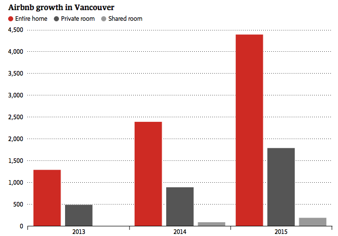
3. Assume 3000 landlords decide to switch from renting to Airbnb, show the impact of the changes on Figure CS3 b. Label the new equilibrium price and quantity.

Note that Airbnb has been adamant that short-term rentals have had a neglible impact on the housing market, citing that in Vancouver only 320 hosts rent out thier properties often enough to make more money that long term rentals. That represents only 0.11% of the total housing units. In Victoria, that would mean only 25 units are affected by short-term rentals.

Tom Davidoff , a  University of B.C. business professor, said t he general public frequently looks at the fact that Airbnb is popular in expensive neighbourhoods and concludes that it is Airbnb that drives up rents there. But, he said, those neighbourhoods were expensive anyway and the impact of Airbnb taking a certain slice of the available stock is minimal.

Read more about Airbnb’s supposed impact on the market.

Another factor that has had an impact on the rental market is the inability of many young Canadians to buy homes. Not only have house prices skyrocketed, but more are burdened by student loans out of university. It is estimated that it takes 3 times longer (15 years) to save enough to have a 20% downpayment on a house than it did in 1976. This reduction in Canadians mortgaging a home has caused an increasing amount to enter the market.

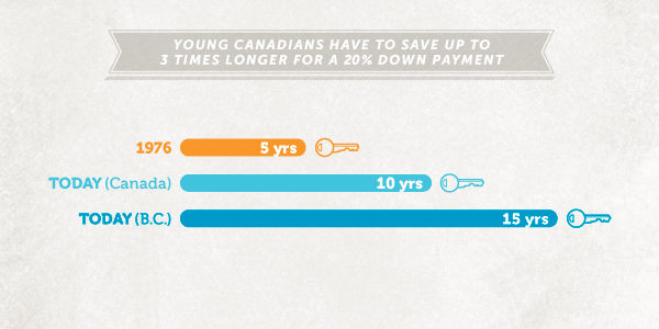
Read more about the increasing squeeze on millennials.

4. Assume 9000 new renters enter the market instead of mortgaging homes, show the impact of the changes on Figure CS3 b.  Explain the impact of both the shock from Airbnb and the shock from less housing buyers on equilibrium price and quantity. Do the shocks work together or oppose one another?

In the housing market, prices are slow to adjust, landlords cannot simply raise prices immediately under the Residential Tenancy Act. Landlords can only raise prices when negotiating a new contract. This causes many unjustified evictions from landlords as they want to charge the new equilibrium price. In the short-term, prices stay relatively the same causing shortages or surplus.

5. Assume price remains at the original equilibrium , calculate the magnitude of the shortage or surplus of housing that results. Explain the impact this shortage will have the behaviour of landlords.

The British Columbia government unveiled a $500-million affordable-housing plan targeted at communities that have struggled with a shortage of low-cost housing.  Premier Christy Clark announced her government’s commitment to fund 68 new projects to help address the crisis

Read more about the governments response to the housing crisis.

6. Assume the government wants to bring price back to it’s original level, if it costs $50,000 to increase the number of rental units by one, how much will this cost the government?

Groups have criticized the government response, saying that they have ignored many other avenues that could more easily increase the supply of affordable housing.

7. Read the Executive Summary of the Alliance of BC Students White Paper on Student Housing.

What is the ABCS proposing that could help decrease price in the market? How would this affect supply and/or demand?

In this case study we have shown how microeconomic concepts of supply and demand can be used to understand current events in the news. Do you have a story you think would make a good case study? Contact [email protected] to propose your story.

Principles of Microeconomics Copyright © 2017 by University of Victoria is licensed under a Creative Commons Attribution 4.0 International License , except where otherwise noted.

Share This Book

Connect with Us

• Entertainment
• Gadgets Review
• Government Schemes
• Make Money Online
• Product Review
• Uncategorized

Solving Case Study in Economics: A Complete Guide

case study in economics

Case studies are invaluable in economics education, providing students with real-world scenarios to apply theoretical concepts and analytical skills. However, solving a case study in economics requires a structured approach that combines research, critical thinking, and a deep understanding of economic principles. This post presents a comprehensive guide on effectively solving a case study in economics , ensuring a thorough analysis and a grasp of practical implications.

Understanding the Case Study

Read carefully: .

Begin by reading the case study thoroughly. Pay attention to the details, context, and objectives presented. Identify the main issues, stakeholders, and the economic concepts at play.

Define the Problem: 

Clearly define the economic problem or challenge presented in the case study. What are the fundamental problems that ought to be handled? Understanding the problem is crucial before proceeding with analysis.Identify the central economic problem or challenge that the case study presents. This could involve issues related to demand and supply, market structures, externalities, government interventions, or any other economic concept.

Gathering Relevant Information

Research: .

Conduct thorough research to gather additional information relevant to the case study. This may involve exploring economic theories, statistical data, and industry trends. Reliable sources such as academic journals, government reports, and reputable news outlets are valuable.

Identify Variables: 

Identify the variables affecting the situation presented in the case study. These could include economic indicators, market conditions, government policies, etc.

Read also: How Trademark Registration Can Help in Business

Applying Economic Concepts

Use relevant theories: .

Apply relevant economic theories and concepts to analyze the case study. Consider concepts like supply and demand, elasticity, market structure, cost analysis, and utility theory, depending on the case context.

Quantitative Analysis:  

If applicable, use quantitative methods such as calculations, graphs, and charts to illustrate your analysis. These tools can help visualize economic relationships and trends.

Data Interpretation

Cause and effect:.

 Identify the cause-and-effect relationships driving the economic situation in the case study. Analyze how changes in one variable can impact others and lead to specific outcomes.

Consider Alternatives: 

Explore solutions or strategies to address the issues presented. Consider the possible benefits and drawbacks of each option.

Making Recommendations

Informed decisions: .

Based on your analysis, make informed recommendations for addressing the challenges outlined in the case study in economics. Your recommendations should be rooted in economic theories and supported by your gathered data.

Justify Your Recommendations: 

Clearly explain the rationale behind your recommendations. How will they positively impact the stakeholders involved? Justify your choices with economic logic.

Read also: Best Practices for Workday Financial Management Integration

Tips for Success

Practice: .

The more case studies you solve, the more comfortable you’ll become with the process. Practice hones your analytical skills and enables you to apply economic concepts effectively.

Collaborate: 

Engage in discussions with peers or instructors. Collaborative analysis can offer diverse perspectives and deepen your understanding of the case.

Real-World Context: 

Relate the case study to real-world economic scenarios. Understanding the practical implications of your analysis adds depth to your recommendations.

Stay Updated:

 Case study in economics is a dynamic field. Stay updated with current economic trends, policy changes, and market developments to enhance the relevance of your analysis.

Read the Case Thoroughly

Begin by reading the case study attentively. Familiarize yourself with the context, characters, and economic issues presented. Take notes as you read to highlight key information and identify the main problems.

 Apply Relevant Economic Concepts

Next, apply the economic concepts and theories you’ve learned in your coursework to the identified problem. Consider how concepts like elasticity, opportunity cost, marginal analysis, and cost-benefit analysis can be applied to the situation.

 Collect Data and Information

Gather relevant data and information that can support your analysis. This may include statistical data, market trends, historical information, and other relevant sources that substantiate your arguments.

Analyze and Evaluate

Conduct a thorough analysis of the situation. Identify the factors contributing to the problem and evaluate their impact. Use graphs, charts, and diagrams to represent your analysis and provide clarity visually.

 Explore Alternatives

Generate possible solutions or alternatives to address the identified problem. Consider the pros and cons of each solution, keeping in mind economic feasibility, ethical implications, and potential outcomes.

 Apply Economic Theories

When formulating solutions, apply economic theories and principles that align with the situation. For instance, if you’re dealing with a market failure, explore how government intervention or corrective measures can be applied based on economic theories like externalities or public goods.

Quantitative Analysis

If applicable, perform quantitative analysis using relevant mathematical or statistical tools. This could involve calculating elasticity break-even points or analyzing cost structures to support your recommendations.

 Justify Your Recommendations

Ensure that your solutions are well-justified and backed by solid economic reasoning. Explain how each solution addresses the problem and aligns with economic theories.

 Consider Real-World Constraints

Acknowledge any real-world constraints that might affect the implementation of your recommendations. This could include budgetary limitations, political considerations, or social factors.

Solving an case study in economics writing is an enriching experience that bridges theory and practice. It requires a structured approach, from understanding the case to making well-informed recommendations. By thoroughly analyzing the economic concepts, interpreting data, and applying relevant theories, you can arrive at strategic solutions that align with economic principles.

Leave a Reply Cancel reply

Your email address will not be published. Required fields are marked *

Save my name, email, and website in this browser for the next time I comment.

Related News

How to migrate from Wix to WordPress – Ultimate Guide

7 Best Team Collaboration Tools for Remote & In-Person

You may have missed.

How to Personalize Custom Boxes for Special Occasions?

How to Fix NVIDIA GeForce Experience Error Code 0x0003

Style Mastery: Essential Tips for Every Woman’s Occasion

Creating High-Performance Teams for Success 

Health and Insurance Bridging the Gap of Technology

UBO Verification: Understand the Ultimate Beneficial Owners 

Thank you for visiting nature.com. You are using a browser version with limited support for CSS. To obtain the best experience, we recommend you use a more up to date browser (or turn off compatibility mode in Internet Explorer). In the meantime, to ensure continued support, we are displaying the site without styles and JavaScript.

• View all journals
• My Account Login
• Explore content
• About the journal
• Publish with us
• Sign up for alerts
• Open access
• Published: 17 April 2024

The economic commitment of climate change

• Maximilian Kotz   ORCID: orcid.org/0000-0003-2564-5043 1 , 2 ,
• Anders Levermann   ORCID: orcid.org/0000-0003-4432-4704 1 , 2 &
• Leonie Wenz   ORCID: orcid.org/0000-0002-8500-1568 1 , 3  

Nature volume  628 ,  pages 551–557 ( 2024 ) Cite this article

82k Accesses

3427 Altmetric

Metrics details

• Environmental economics
• Environmental health
• Interdisciplinary studies
• Projection and prediction

Global projections of macroeconomic climate-change damages typically consider impacts from average annual and national temperatures over long time horizons 1 , 2 , 3 , 4 , 5 , 6 . Here we use recent empirical findings from more than 1,600 regions worldwide over the past 40 years to project sub-national damages from temperature and precipitation, including daily variability and extremes 7 , 8 . Using an empirical approach that provides a robust lower bound on the persistence of impacts on economic growth, we find that the world economy is committed to an income reduction of 19% within the next 26 years independent of future emission choices (relative to a baseline without climate impacts, likely range of 11–29% accounting for physical climate and empirical uncertainty). These damages already outweigh the mitigation costs required to limit global warming to 2 °C by sixfold over this near-term time frame and thereafter diverge strongly dependent on emission choices. Committed damages arise predominantly through changes in average temperature, but accounting for further climatic components raises estimates by approximately 50% and leads to stronger regional heterogeneity. Committed losses are projected for all regions except those at very high latitudes, at which reductions in temperature variability bring benefits. The largest losses are committed at lower latitudes in regions with lower cumulative historical emissions and lower present-day income.

Similar content being viewed by others

Climate damage projections beyond annual temperature

Investment incentive reduced by climate damages can be restored by optimal policy

Climate economics support for the UN climate targets

Projections of the macroeconomic damage caused by future climate change are crucial to informing public and policy debates about adaptation, mitigation and climate justice. On the one hand, adaptation against climate impacts must be justified and planned on the basis of an understanding of their future magnitude and spatial distribution 9 . This is also of importance in the context of climate justice 10 , as well as to key societal actors, including governments, central banks and private businesses, which increasingly require the inclusion of climate risks in their macroeconomic forecasts to aid adaptive decision-making 11 , 12 . On the other hand, climate mitigation policy such as the Paris Climate Agreement is often evaluated by balancing the costs of its implementation against the benefits of avoiding projected physical damages. This evaluation occurs both formally through cost–benefit analyses 1 , 4 , 5 , 6 , as well as informally through public perception of mitigation and damage costs 13 .

Projections of future damages meet challenges when informing these debates, in particular the human biases relating to uncertainty and remoteness that are raised by long-term perspectives 14 . Here we aim to overcome such challenges by assessing the extent of economic damages from climate change to which the world is already committed by historical emissions and socio-economic inertia (the range of future emission scenarios that are considered socio-economically plausible 15 ). Such a focus on the near term limits the large uncertainties about diverging future emission trajectories, the resulting long-term climate response and the validity of applying historically observed climate–economic relations over long timescales during which socio-technical conditions may change considerably. As such, this focus aims to simplify the communication and maximize the credibility of projected economic damages from future climate change.

In projecting the future economic damages from climate change, we make use of recent advances in climate econometrics that provide evidence for impacts on sub-national economic growth from numerous components of the distribution of daily temperature and precipitation 3 , 7 , 8 . Using fixed-effects panel regression models to control for potential confounders, these studies exploit within-region variation in local temperature and precipitation in a panel of more than 1,600 regions worldwide, comprising climate and income data over the past 40 years, to identify the plausibly causal effects of changes in several climate variables on economic productivity 16 , 17 . Specifically, macroeconomic impacts have been identified from changing daily temperature variability, total annual precipitation, the annual number of wet days and extreme daily rainfall that occur in addition to those already identified from changing average temperature 2 , 3 , 18 . Moreover, regional heterogeneity in these effects based on the prevailing local climatic conditions has been found using interactions terms. The selection of these climate variables follows micro-level evidence for mechanisms related to the impacts of average temperatures on labour and agricultural productivity 2 , of temperature variability on agricultural productivity and health 7 , as well as of precipitation on agricultural productivity, labour outcomes and flood damages 8 (see Extended Data Table 1 for an overview, including more detailed references). References  7 , 8 contain a more detailed motivation for the use of these particular climate variables and provide extensive empirical tests about the robustness and nature of their effects on economic output, which are summarized in Methods . By accounting for these extra climatic variables at the sub-national level, we aim for a more comprehensive description of climate impacts with greater detail across both time and space.

Constraining the persistence of impacts

A key determinant and source of discrepancy in estimates of the magnitude of future climate damages is the extent to which the impact of a climate variable on economic growth rates persists. The two extreme cases in which these impacts persist indefinitely or only instantaneously are commonly referred to as growth or level effects 19 , 20 (see Methods section ‘Empirical model specification: fixed-effects distributed lag models’ for mathematical definitions). Recent work shows that future damages from climate change depend strongly on whether growth or level effects are assumed 20 . Following refs.  2 , 18 , we provide constraints on this persistence by using distributed lag models to test the significance of delayed effects separately for each climate variable. Notably, and in contrast to refs.  2 , 18 , we use climate variables in their first-differenced form following ref.  3 , implying a dependence of the growth rate on a change in climate variables. This choice means that a baseline specification without any lags constitutes a model prior of purely level effects, in which a permanent change in the climate has only an instantaneous effect on the growth rate 3 , 19 , 21 . By including lags, one can then test whether any effects may persist further. This is in contrast to the specification used by refs.  2 , 18 , in which climate variables are used without taking the first difference, implying a dependence of the growth rate on the level of climate variables. In this alternative case, the baseline specification without any lags constitutes a model prior of pure growth effects, in which a change in climate has an infinitely persistent effect on the growth rate. Consequently, including further lags in this alternative case tests whether the initial growth impact is recovered 18 , 19 , 21 . Both of these specifications suffer from the limiting possibility that, if too few lags are included, one might falsely accept the model prior. The limitations of including a very large number of lags, including loss of data and increasing statistical uncertainty with an increasing number of parameters, mean that such a possibility is likely. By choosing a specification in which the model prior is one of level effects, our approach is therefore conservative by design, avoiding assumptions of infinite persistence of climate impacts on growth and instead providing a lower bound on this persistence based on what is observable empirically (see Methods section ‘Empirical model specification: fixed-effects distributed lag models’ for further exposition of this framework). The conservative nature of such a choice is probably the reason that ref.  19 finds much greater consistency between the impacts projected by models that use the first difference of climate variables, as opposed to their levels.

We begin our empirical analysis of the persistence of climate impacts on growth using ten lags of the first-differenced climate variables in fixed-effects distributed lag models. We detect substantial effects on economic growth at time lags of up to approximately 8–10 years for the temperature terms and up to approximately 4 years for the precipitation terms (Extended Data Fig. 1 and Extended Data Table 2 ). Furthermore, evaluation by means of information criteria indicates that the inclusion of all five climate variables and the use of these numbers of lags provide a preferable trade-off between best-fitting the data and including further terms that could cause overfitting, in comparison with model specifications excluding climate variables or including more or fewer lags (Extended Data Fig. 3 , Supplementary Methods Section  1 and Supplementary Table 1 ). We therefore remove statistically insignificant terms at later lags (Supplementary Figs. 1 – 3 and Supplementary Tables 2 – 4 ). Further tests using Monte Carlo simulations demonstrate that the empirical models are robust to autocorrelation in the lagged climate variables (Supplementary Methods Section  2 and Supplementary Figs. 4 and 5 ), that information criteria provide an effective indicator for lag selection (Supplementary Methods Section  2 and Supplementary Fig. 6 ), that the results are robust to concerns of imperfect multicollinearity between climate variables and that including several climate variables is actually necessary to isolate their separate effects (Supplementary Methods Section  3 and Supplementary Fig. 7 ). We provide a further robustness check using a restricted distributed lag model to limit oscillations in the lagged parameter estimates that may result from autocorrelation, finding that it provides similar estimates of cumulative marginal effects to the unrestricted model (Supplementary Methods Section 4 and Supplementary Figs. 8 and 9 ). Finally, to explicitly account for any outstanding uncertainty arising from the precise choice of the number of lags, we include empirical models with marginally different numbers of lags in the error-sampling procedure of our projection of future damages. On the basis of the lag-selection procedure (the significance of lagged terms in Extended Data Fig. 1 and Extended Data Table 2 , as well as information criteria in Extended Data Fig. 3 ), we sample from models with eight to ten lags for temperature and four for precipitation (models shown in Supplementary Figs. 1 – 3 and Supplementary Tables 2 – 4 ). In summary, this empirical approach to constrain the persistence of climate impacts on economic growth rates is conservative by design in avoiding assumptions of infinite persistence, but nevertheless provides a lower bound on the extent of impact persistence that is robust to the numerous tests outlined above.

Committed damages until mid-century

We combine these empirical economic response functions (Supplementary Figs. 1 – 3 and Supplementary Tables 2 – 4 ) with an ensemble of 21 climate models (see Supplementary Table 5 ) from the Coupled Model Intercomparison Project Phase 6 (CMIP-6) 22 to project the macroeconomic damages from these components of physical climate change (see Methods for further details). Bias-adjusted climate models that provide a highly accurate reproduction of observed climatological patterns with limited uncertainty (Supplementary Table 6 ) are used to avoid introducing biases in the projections. Following a well-developed literature 2 , 3 , 19 , these projections do not aim to provide a prediction of future economic growth. Instead, they are a projection of the exogenous impact of future climate conditions on the economy relative to the baselines specified by socio-economic projections, based on the plausibly causal relationships inferred by the empirical models and assuming ceteris paribus. Other exogenous factors relevant for the prediction of economic output are purposefully assumed constant.

A Monte Carlo procedure that samples from climate model projections, empirical models with different numbers of lags and model parameter estimates (obtained by 1,000 block-bootstrap resamples of each of the regressions in Supplementary Figs. 1 – 3 and Supplementary Tables 2 – 4 ) is used to estimate the combined uncertainty from these sources. Given these uncertainty distributions, we find that projected global damages are statistically indistinguishable across the two most extreme emission scenarios until 2049 (at the 5% significance level; Fig. 1 ). As such, the climate damages occurring before this time constitute those to which the world is already committed owing to the combination of past emissions and the range of future emission scenarios that are considered socio-economically plausible 15 . These committed damages comprise a permanent income reduction of 19% on average globally (population-weighted average) in comparison with a baseline without climate-change impacts (with a likely range of 11–29%, following the likelihood classification adopted by the Intergovernmental Panel on Climate Change (IPCC); see caption of Fig. 1 ). Even though levels of income per capita generally still increase relative to those of today, this constitutes a permanent income reduction for most regions, including North America and Europe (each with median income reductions of approximately 11%) and with South Asia and Africa being the most strongly affected (each with median income reductions of approximately 22%; Fig. 1 ). Under a middle-of-the road scenario of future income development (SSP2, in which SSP stands for Shared Socio-economic Pathway), this corresponds to global annual damages in 2049 of 38 trillion in 2005 international dollars (likely range of 19–59 trillion 2005 international dollars). Compared with empirical specifications that assume pure growth or pure level effects, our preferred specification that provides a robust lower bound on the extent of climate impact persistence produces damages between these two extreme assumptions (Extended Data Fig. 3 ).

Estimates of the projected reduction in income per capita from changes in all climate variables based on empirical models of climate impacts on economic output with a robust lower bound on their persistence (Extended Data Fig. 1 ) under a low-emission scenario compatible with the 2 °C warming target and a high-emission scenario (SSP2-RCP2.6 and SSP5-RCP8.5, respectively) are shown in purple and orange, respectively. Shading represents the 34% and 10% confidence intervals reflecting the likely and very likely ranges, respectively (following the likelihood classification adopted by the IPCC), having estimated uncertainty from a Monte Carlo procedure, which samples the uncertainty from the choice of physical climate models, empirical models with different numbers of lags and bootstrapped estimates of the regression parameters shown in Supplementary Figs. 1 – 3 . Vertical dashed lines show the time at which the climate damages of the two emission scenarios diverge at the 5% and 1% significance levels based on the distribution of differences between emission scenarios arising from the uncertainty sampling discussed above. Note that uncertainty in the difference of the two scenarios is smaller than the combined uncertainty of the two respective scenarios because samples of the uncertainty (climate model and empirical model choice, as well as model parameter bootstrap) are consistent across the two emission scenarios, hence the divergence of damages occurs while the uncertainty bounds of the two separate damage scenarios still overlap. Estimates of global mitigation costs from the three IAMs that provide results for the SSP2 baseline and SSP2-RCP2.6 scenario are shown in light green in the top panel, with the median of these estimates shown in bold.

Damages already outweigh mitigation costs

We compare the damages to which the world is committed over the next 25 years to estimates of the mitigation costs required to achieve the Paris Climate Agreement. Taking estimates of mitigation costs from the three integrated assessment models (IAMs) in the IPCC AR6 database 23 that provide results under comparable scenarios (SSP2 baseline and SSP2-RCP2.6, in which RCP stands for Representative Concentration Pathway), we find that the median committed climate damages are larger than the median mitigation costs in 2050 (six trillion in 2005 international dollars) by a factor of approximately six (note that estimates of mitigation costs are only provided every 10 years by the IAMs and so a comparison in 2049 is not possible). This comparison simply aims to compare the magnitude of future damages against mitigation costs, rather than to conduct a formal cost–benefit analysis of transitioning from one emission path to another. Formal cost–benefit analyses typically find that the net benefits of mitigation only emerge after 2050 (ref.  5 ), which may lead some to conclude that physical damages from climate change are simply not large enough to outweigh mitigation costs until the second half of the century. Our simple comparison of their magnitudes makes clear that damages are actually already considerably larger than mitigation costs and the delayed emergence of net mitigation benefits results primarily from the fact that damages across different emission paths are indistinguishable until mid-century (Fig. 1 ).

Although these near-term damages constitute those to which the world is already committed, we note that damage estimates diverge strongly across emission scenarios after 2049, conveying the clear benefits of mitigation from a purely economic point of view that have been emphasized in previous studies 4 , 24 . As well as the uncertainties assessed in Fig. 1 , these conclusions are robust to structural choices, such as the timescale with which changes in the moderating variables of the empirical models are estimated (Supplementary Figs. 10 and 11 ), as well as the order in which one accounts for the intertemporal and international components of currency comparison (Supplementary Fig. 12 ; see Methods for further details).

Damages from variability and extremes

Committed damages primarily arise through changes in average temperature (Fig. 2 ). This reflects the fact that projected changes in average temperature are larger than those in other climate variables when expressed as a function of their historical interannual variability (Extended Data Fig. 4 ). Because the historical variability is that on which the empirical models are estimated, larger projected changes in comparison with this variability probably lead to larger future impacts in a purely statistical sense. From a mechanistic perspective, one may plausibly interpret this result as implying that future changes in average temperature are the most unprecedented from the perspective of the historical fluctuations to which the economy is accustomed and therefore will cause the most damage. This insight may prove useful in terms of guiding adaptation measures to the sources of greatest damage.

Estimates of the median projected reduction in sub-national income per capita across emission scenarios (SSP2-RCP2.6 and SSP2-RCP8.5) as well as climate model, empirical model and model parameter uncertainty in the year in which climate damages diverge at the 5% level (2049, as identified in Fig. 1 ). a , Impacts arising from all climate variables. b – f , Impacts arising separately from changes in annual mean temperature ( b ), daily temperature variability ( c ), total annual precipitation ( d ), the annual number of wet days (>1 mm) ( e ) and extreme daily rainfall ( f ) (see Methods for further definitions). Data on national administrative boundaries are obtained from the GADM database version 3.6 and are freely available for academic use ( https://gadm.org/ ).

Nevertheless, future damages based on empirical models that consider changes in annual average temperature only and exclude the other climate variables constitute income reductions of only 13% in 2049 (Extended Data Fig. 5a , likely range 5–21%). This suggests that accounting for the other components of the distribution of temperature and precipitation raises net damages by nearly 50%. This increase arises through the further damages that these climatic components cause, but also because their inclusion reveals a stronger negative economic response to average temperatures (Extended Data Fig. 5b ). The latter finding is consistent with our Monte Carlo simulations, which suggest that the magnitude of the effect of average temperature on economic growth is underestimated unless accounting for the impacts of other correlated climate variables (Supplementary Fig. 7 ).

In terms of the relative contributions of the different climatic components to overall damages, we find that accounting for daily temperature variability causes the largest increase in overall damages relative to empirical frameworks that only consider changes in annual average temperature (4.9 percentage points, likely range 2.4–8.7 percentage points, equivalent to approximately 10 trillion international dollars). Accounting for precipitation causes smaller increases in overall damages, which are—nevertheless—equivalent to approximately 1.2 trillion international dollars: 0.01 percentage points (−0.37–0.33 percentage points), 0.34 percentage points (0.07–0.90 percentage points) and 0.36 percentage points (0.13–0.65 percentage points) from total annual precipitation, the number of wet days and extreme daily precipitation, respectively. Moreover, climate models seem to underestimate future changes in temperature variability 25 and extreme precipitation 26 , 27 in response to anthropogenic forcing as compared with that observed historically, suggesting that the true impacts from these variables may be larger.

The distribution of committed damages

The spatial distribution of committed damages (Fig. 2a ) reflects a complex interplay between the patterns of future change in several climatic components and those of historical economic vulnerability to changes in those variables. Damages resulting from increasing annual mean temperature (Fig. 2b ) are negative almost everywhere globally, and larger at lower latitudes in regions in which temperatures are already higher and economic vulnerability to temperature increases is greatest (see the response heterogeneity to mean temperature embodied in Extended Data Fig. 1a ). This occurs despite the amplified warming projected at higher latitudes 28 , suggesting that regional heterogeneity in economic vulnerability to temperature changes outweighs heterogeneity in the magnitude of future warming (Supplementary Fig. 13a ). Economic damages owing to daily temperature variability (Fig. 2c ) exhibit a strong latitudinal polarisation, primarily reflecting the physical response of daily variability to greenhouse forcing in which increases in variability across lower latitudes (and Europe) contrast decreases at high latitudes 25 (Supplementary Fig. 13b ). These two temperature terms are the dominant determinants of the pattern of overall damages (Fig. 2a ), which exhibits a strong polarity with damages across most of the globe except at the highest northern latitudes. Future changes in total annual precipitation mainly bring economic benefits except in regions of drying, such as the Mediterranean and central South America (Fig. 2d and Supplementary Fig. 13c ), but these benefits are opposed by changes in the number of wet days, which produce damages with a similar pattern of opposite sign (Fig. 2e and Supplementary Fig. 13d ). By contrast, changes in extreme daily rainfall produce damages in all regions, reflecting the intensification of daily rainfall extremes over global land areas 29 , 30 (Fig. 2f and Supplementary Fig. 13e ).

The spatial distribution of committed damages implies considerable injustice along two dimensions: culpability for the historical emissions that have caused climate change and pre-existing levels of socio-economic welfare. Spearman’s rank correlations indicate that committed damages are significantly larger in countries with smaller historical cumulative emissions, as well as in regions with lower current income per capita (Fig. 3 ). This implies that those countries that will suffer the most from the damages already committed are those that are least responsible for climate change and which also have the least resources to adapt to it.

Estimates of the median projected change in national income per capita across emission scenarios (RCP2.6 and RCP8.5) as well as climate model, empirical model and model parameter uncertainty in the year in which climate damages diverge at the 5% level (2049, as identified in Fig. 1 ) are plotted against cumulative national emissions per capita in 2020 (from the Global Carbon Project) and coloured by national income per capita in 2020 (from the World Bank) in a and vice versa in b . In each panel, the size of each scatter point is weighted by the national population in 2020 (from the World Bank). Inset numbers indicate the Spearman’s rank correlation ρ and P -values for a hypothesis test whose null hypothesis is of no correlation, as well as the Spearman’s rank correlation weighted by national population.

To further quantify this heterogeneity, we assess the difference in committed damages between the upper and lower quartiles of regions when ranked by present income levels and historical cumulative emissions (using a population weighting to both define the quartiles and estimate the group averages). On average, the quartile of countries with lower income are committed to an income loss that is 8.9 percentage points (or 61%) greater than the upper quartile (Extended Data Fig. 6 ), with a likely range of 3.8–14.7 percentage points across the uncertainty sampling of our damage projections (following the likelihood classification adopted by the IPCC). Similarly, the quartile of countries with lower historical cumulative emissions are committed to an income loss that is 6.9 percentage points (or 40%) greater than the upper quartile, with a likely range of 0.27–12 percentage points. These patterns reemphasize the prevalence of injustice in climate impacts 31 , 32 , 33 in the context of the damages to which the world is already committed by historical emissions and socio-economic inertia.

Contextualizing the magnitude of damages

The magnitude of projected economic damages exceeds previous literature estimates 2 , 3 , arising from several developments made on previous approaches. Our estimates are larger than those of ref.  2 (see first row of Extended Data Table 3 ), primarily because of the facts that sub-national estimates typically show a steeper temperature response (see also refs.  3 , 34 ) and that accounting for other climatic components raises damage estimates (Extended Data Fig. 5 ). However, we note that our empirical approach using first-differenced climate variables is conservative compared with that of ref.  2 in regard to the persistence of climate impacts on growth (see introduction and Methods section ‘Empirical model specification: fixed-effects distributed lag models’), an important determinant of the magnitude of long-term damages 19 , 21 . Using a similar empirical specification to ref.  2 , which assumes infinite persistence while maintaining the rest of our approach (sub-national data and further climate variables), produces considerably larger damages (purple curve of Extended Data Fig. 3 ). Compared with studies that do take the first difference of climate variables 3 , 35 , our estimates are also larger (see second and third rows of Extended Data Table 3 ). The inclusion of further climate variables (Extended Data Fig. 5 ) and a sufficient number of lags to more adequately capture the extent of impact persistence (Extended Data Figs. 1 and 2 ) are the main sources of this difference, as is the use of specifications that capture nonlinearities in the temperature response when compared with ref.  35 . In summary, our estimates develop on previous studies by incorporating the latest data and empirical insights 7 , 8 , as well as in providing a robust empirical lower bound on the persistence of impacts on economic growth, which constitutes a middle ground between the extremes of the growth-versus-levels debate 19 , 21 (Extended Data Fig. 3 ).

Compared with the fraction of variance explained by the empirical models historically (<5%), the projection of reductions in income of 19% may seem large. This arises owing to the fact that projected changes in climatic conditions are much larger than those that were experienced historically, particularly for changes in average temperature (Extended Data Fig. 4 ). As such, any assessment of future climate-change impacts necessarily requires an extrapolation outside the range of the historical data on which the empirical impact models were evaluated. Nevertheless, these models constitute the most state-of-the-art methods for inference of plausibly causal climate impacts based on observed data. Moreover, we take explicit steps to limit out-of-sample extrapolation by capping the moderating variables of the interaction terms at the 95th percentile of the historical distribution (see Methods ). This avoids extrapolating the marginal effects outside what was observed historically. Given the nonlinear response of economic output to annual mean temperature (Extended Data Fig. 1 and Extended Data Table 2 ), this is a conservative choice that limits the magnitude of damages that we project. Furthermore, back-of-the-envelope calculations indicate that the projected damages are consistent with the magnitude and patterns of historical economic development (see Supplementary Discussion Section  5 ).

Missing impacts and spatial spillovers

Despite assessing several climatic components from which economic impacts have recently been identified 3 , 7 , 8 , this assessment of aggregate climate damages should not be considered comprehensive. Important channels such as impacts from heatwaves 31 , sea-level rise 36 , tropical cyclones 37 and tipping points 38 , 39 , as well as non-market damages such as those to ecosystems 40 and human health 41 , are not considered in these estimates. Sea-level rise is unlikely to be feasibly incorporated into empirical assessments such as this because historical sea-level variability is mostly small. Non-market damages are inherently intractable within our estimates of impacts on aggregate monetary output and estimates of these impacts could arguably be considered as extra to those identified here. Recent empirical work suggests that accounting for these channels would probably raise estimates of these committed damages, with larger damages continuing to arise in the global south 31 , 36 , 37 , 38 , 39 , 40 , 41 , 42 .

Moreover, our main empirical analysis does not explicitly evaluate the potential for impacts in local regions to produce effects that ‘spill over’ into other regions. Such effects may further mitigate or amplify the impacts we estimate, for example, if companies relocate production from one affected region to another or if impacts propagate along supply chains. The current literature indicates that trade plays a substantial role in propagating spillover effects 43 , 44 , making their assessment at the sub-national level challenging without available data on sub-national trade dependencies. Studies accounting for only spatially adjacent neighbours indicate that negative impacts in one region induce further negative impacts in neighbouring regions 45 , 46 , 47 , 48 , suggesting that our projected damages are probably conservative by excluding these effects. In Supplementary Fig. 14 , we assess spillovers from neighbouring regions using a spatial-lag model. For simplicity, this analysis excludes temporal lags, focusing only on contemporaneous effects. The results show that accounting for spatial spillovers can amplify the overall magnitude, and also the heterogeneity, of impacts. Consistent with previous literature, this indicates that the overall magnitude (Fig. 1 ) and heterogeneity (Fig. 3 ) of damages that we project in our main specification may be conservative without explicitly accounting for spillovers. We note that further analysis that addresses both spatially and trade-connected spillovers, while also accounting for delayed impacts using temporal lags, would be necessary to adequately address this question fully. These approaches offer fruitful avenues for further research but are beyond the scope of this manuscript, which primarily aims to explore the impacts of different climate conditions and their persistence.

Policy implications

We find that the economic damages resulting from climate change until 2049 are those to which the world economy is already committed and that these greatly outweigh the costs required to mitigate emissions in line with the 2 °C target of the Paris Climate Agreement (Fig. 1 ). This assessment is complementary to formal analyses of the net costs and benefits associated with moving from one emission path to another, which typically find that net benefits of mitigation only emerge in the second half of the century 5 . Our simple comparison of the magnitude of damages and mitigation costs makes clear that this is primarily because damages are indistinguishable across emissions scenarios—that is, committed—until mid-century (Fig. 1 ) and that they are actually already much larger than mitigation costs. For simplicity, and owing to the availability of data, we compare damages to mitigation costs at the global level. Regional estimates of mitigation costs may shed further light on the national incentives for mitigation to which our results already hint, of relevance for international climate policy. Although these damages are committed from a mitigation perspective, adaptation may provide an opportunity to reduce them. Moreover, the strong divergence of damages after mid-century reemphasizes the clear benefits of mitigation from a purely economic perspective, as highlighted in previous studies 1 , 4 , 6 , 24 .

Historical climate data

Historical daily 2-m temperature and precipitation totals (in mm) are obtained for the period 1979–2019 from the W5E5 database. The W5E5 dataset comes from ERA-5, a state-of-the-art reanalysis of historical observations, but has been bias-adjusted by applying version 2.0 of the WATCH Forcing Data to ERA-5 reanalysis data and precipitation data from version 2.3 of the Global Precipitation Climatology Project to better reflect ground-based measurements 49 , 50 , 51 . We obtain these data on a 0.5° × 0.5° grid from the Inter-Sectoral Impact Model Intercomparison Project (ISIMIP) database. Notably, these historical data have been used to bias-adjust future climate projections from CMIP-6 (see the following section), ensuring consistency between the distribution of historical daily weather on which our empirical models were estimated and the climate projections used to estimate future damages. These data are publicly available from the ISIMIP database. See refs.  7 , 8 for robustness tests of the empirical models to the choice of climate data reanalysis products.

Future climate data

Daily 2-m temperature and precipitation totals (in mm) are taken from 21 climate models participating in CMIP-6 under a high (RCP8.5) and a low (RCP2.6) greenhouse gas emission scenario from 2015 to 2100. The data have been bias-adjusted and statistically downscaled to a common half-degree grid to reflect the historical distribution of daily temperature and precipitation of the W5E5 dataset using the trend-preserving method developed by the ISIMIP 50 , 52 . As such, the climate model data reproduce observed climatological patterns exceptionally well (Supplementary Table 5 ). Gridded data are publicly available from the ISIMIP database.

Historical economic data

Historical economic data come from the DOSE database of sub-national economic output 53 . We use a recent revision to the DOSE dataset that provides data across 83 countries, 1,660 sub-national regions with varying temporal coverage from 1960 to 2019. Sub-national units constitute the first administrative division below national, for example, states for the USA and provinces for China. Data come from measures of gross regional product per capita (GRPpc) or income per capita in local currencies, reflecting the values reported in national statistical agencies, yearbooks and, in some cases, academic literature. We follow previous literature 3 , 7 , 8 , 54 and assess real sub-national output per capita by first converting values from local currencies to US dollars to account for diverging national inflationary tendencies and then account for US inflation using a US deflator. Alternatively, one might first account for national inflation and then convert between currencies. Supplementary Fig. 12 demonstrates that our conclusions are consistent when accounting for price changes in the reversed order, although the magnitude of estimated damages varies. See the documentation of the DOSE dataset for further discussion of these choices. Conversions between currencies are conducted using exchange rates from the FRED database of the Federal Reserve Bank of St. Louis 55 and the national deflators from the World Bank 56 .

Future socio-economic data

Baseline gridded gross domestic product (GDP) and population data for the period 2015–2100 are taken from the middle-of-the-road scenario SSP2 (ref.  15 ). Population data have been downscaled to a half-degree grid by the ISIMIP following the methodologies of refs.  57 , 58 , which we then aggregate to the sub-national level of our economic data using the spatial aggregation procedure described below. Because current methodologies for downscaling the GDP of the SSPs use downscaled population to do so, per-capita estimates of GDP with a realistic distribution at the sub-national level are not readily available for the SSPs. We therefore use national-level GDP per capita (GDPpc) projections for all sub-national regions of a given country, assuming homogeneity within countries in terms of baseline GDPpc. Here we use projections that have been updated to account for the impact of the COVID-19 pandemic on the trajectory of future income, while remaining consistent with the long-term development of the SSPs 59 . The choice of baseline SSP alters the magnitude of projected climate damages in monetary terms, but when assessed in terms of percentage change from the baseline, the choice of socio-economic scenario is inconsequential. Gridded SSP population data and national-level GDPpc data are publicly available from the ISIMIP database. Sub-national estimates as used in this study are available in the code and data replication files.

Climate variables

Following recent literature 3 , 7 , 8 , we calculate an array of climate variables for which substantial impacts on macroeconomic output have been identified empirically, supported by further evidence at the micro level for plausible underlying mechanisms. See refs.  7 , 8 for an extensive motivation for the use of these particular climate variables and for detailed empirical tests on the nature and robustness of their effects on economic output. To summarize, these studies have found evidence for independent impacts on economic growth rates from annual average temperature, daily temperature variability, total annual precipitation, the annual number of wet days and extreme daily rainfall. Assessments of daily temperature variability were motivated by evidence of impacts on agricultural output and human health, as well as macroeconomic literature on the impacts of volatility on growth when manifest in different dimensions, such as government spending, exchange rates and even output itself 7 . Assessments of precipitation impacts were motivated by evidence of impacts on agricultural productivity, metropolitan labour outcomes and conflict, as well as damages caused by flash flooding 8 . See Extended Data Table 1 for detailed references to empirical studies of these physical mechanisms. Marked impacts of daily temperature variability, total annual precipitation, the number of wet days and extreme daily rainfall on macroeconomic output were identified robustly across different climate datasets, spatial aggregation schemes, specifications of regional time trends and error-clustering approaches. They were also found to be robust to the consideration of temperature extremes 7 , 8 . Furthermore, these climate variables were identified as having independent effects on economic output 7 , 8 , which we further explain here using Monte Carlo simulations to demonstrate the robustness of the results to concerns of imperfect multicollinearity between climate variables (Supplementary Methods Section  2 ), as well as by using information criteria (Supplementary Table 1 ) to demonstrate that including several lagged climate variables provides a preferable trade-off between optimally describing the data and limiting the possibility of overfitting.

We calculate these variables from the distribution of daily, d , temperature, T x , d , and precipitation, P x , d , at the grid-cell, x , level for both the historical and future climate data. As well as annual mean temperature, \({\bar{T}}_{x,y}\) , and annual total precipitation, P x , y , we calculate annual, y , measures of daily temperature variability, \({\widetilde{T}}_{x,y}\) :

the number of wet days, Pwd x , y :

and extreme daily rainfall:

in which T x , d , m , y is the grid-cell-specific daily temperature in month m and year y , \({\bar{T}}_{x,m,{y}}\) is the year and grid-cell-specific monthly, m , mean temperature, D m and D y the number of days in a given month m or year y , respectively, H the Heaviside step function, 1 mm the threshold used to define wet days and P 99.9 x is the 99.9th percentile of historical (1979–2019) daily precipitation at the grid-cell level. Units of the climate measures are degrees Celsius for annual mean temperature and daily temperature variability, millimetres for total annual precipitation and extreme daily precipitation, and simply the number of days for the annual number of wet days.

We also calculated weighted standard deviations of monthly rainfall totals as also used in ref.  8 but do not include them in our projections as we find that, when accounting for delayed effects, their effect becomes statistically indistinct and is better captured by changes in total annual rainfall.

Spatial aggregation

We aggregate grid-cell-level historical and future climate measures, as well as grid-cell-level future GDPpc and population, to the level of the first administrative unit below national level of the GADM database, using an area-weighting algorithm that estimates the portion of each grid cell falling within an administrative boundary. We use this as our baseline specification following previous findings that the effect of area or population weighting at the sub-national level is negligible 7 , 8 .

Empirical model specification: fixed-effects distributed lag models

Following a wide range of climate econometric literature 16 , 60 , we use panel regression models with a selection of fixed effects and time trends to isolate plausibly exogenous variation with which to maximize confidence in a causal interpretation of the effects of climate on economic growth rates. The use of region fixed effects, μ r , accounts for unobserved time-invariant differences between regions, such as prevailing climatic norms and growth rates owing to historical and geopolitical factors. The use of yearly fixed effects, η y , accounts for regionally invariant annual shocks to the global climate or economy such as the El Niño–Southern Oscillation or global recessions. In our baseline specification, we also include region-specific linear time trends, k r y , to exclude the possibility of spurious correlations resulting from common slow-moving trends in climate and growth.

The persistence of climate impacts on economic growth rates is a key determinant of the long-term magnitude of damages. Methods for inferring the extent of persistence in impacts on growth rates have typically used lagged climate variables to evaluate the presence of delayed effects or catch-up dynamics 2 , 18 . For example, consider starting from a model in which a climate condition, C r , y , (for example, annual mean temperature) affects the growth rate, Δlgrp r , y (the first difference of the logarithm of gross regional product) of region r in year y :

which we refer to as a ‘pure growth effects’ model in the main text. Typically, further lags are included,

and the cumulative effect of all lagged terms is evaluated to assess the extent to which climate impacts on growth rates persist. Following ref.  18 , in the case that,

the implication is that impacts on the growth rate persist up to NL years after the initial shock (possibly to a weaker or a stronger extent), whereas if

then the initial impact on the growth rate is recovered after NL years and the effect is only one on the level of output. However, we note that such approaches are limited by the fact that, when including an insufficient number of lags to detect a recovery of the growth rates, one may find equation ( 6 ) to be satisfied and incorrectly assume that a change in climatic conditions affects the growth rate indefinitely. In practice, given a limited record of historical data, including too few lags to confidently conclude in an infinitely persistent impact on the growth rate is likely, particularly over the long timescales over which future climate damages are often projected 2 , 24 . To avoid this issue, we instead begin our analysis with a model for which the level of output, lgrp r , y , depends on the level of a climate variable, C r , y :

Given the non-stationarity of the level of output, we follow the literature 19 and estimate such an equation in first-differenced form as,

which we refer to as a model of ‘pure level effects’ in the main text. This model constitutes a baseline specification in which a permanent change in the climate variable produces an instantaneous impact on the growth rate and a permanent effect only on the level of output. By including lagged variables in this specification,

we are able to test whether the impacts on the growth rate persist any further than instantaneously by evaluating whether α L  > 0 are statistically significantly different from zero. Even though this framework is also limited by the possibility of including too few lags, the choice of a baseline model specification in which impacts on the growth rate do not persist means that, in the case of including too few lags, the framework reverts to the baseline specification of level effects. As such, this framework is conservative with respect to the persistence of impacts and the magnitude of future damages. It naturally avoids assumptions of infinite persistence and we are able to interpret any persistence that we identify with equation ( 9 ) as a lower bound on the extent of climate impact persistence on growth rates. See the main text for further discussion of this specification choice, in particular about its conservative nature compared with previous literature estimates, such as refs.  2 , 18 .

We allow the response to climatic changes to vary across regions, using interactions of the climate variables with historical average (1979–2019) climatic conditions reflecting heterogenous effects identified in previous work 7 , 8 . Following this previous work, the moderating variables of these interaction terms constitute the historical average of either the variable itself or of the seasonal temperature difference, \({\hat{T}}_{r}\) , or annual mean temperature, \({\bar{T}}_{r}\) , in the case of daily temperature variability 7 and extreme daily rainfall, respectively 8 .

The resulting regression equation with N and M lagged variables, respectively, reads:

in which Δlgrp r , y is the annual, regional GRPpc growth rate, measured as the first difference of the logarithm of real GRPpc, following previous work 2 , 3 , 7 , 8 , 18 , 19 . Fixed-effects regressions were run using the fixest package in R (ref.  61 ).

Estimates of the coefficients of interest α i , L are shown in Extended Data Fig. 1 for N  =  M  = 10 lags and for our preferred choice of the number of lags in Supplementary Figs. 1 – 3 . In Extended Data Fig. 1 , errors are shown clustered at the regional level, but for the construction of damage projections, we block-bootstrap the regressions by region 1,000 times to provide a range of parameter estimates with which to sample the projection uncertainty (following refs.  2 , 31 ).

Spatial-lag model

In Supplementary Fig. 14 , we present the results from a spatial-lag model that explores the potential for climate impacts to ‘spill over’ into spatially neighbouring regions. We measure the distance between centroids of each pair of sub-national regions and construct spatial lags that take the average of the first-differenced climate variables and their interaction terms over neighbouring regions that are at distances of 0–500, 500–1,000, 1,000–1,500 and 1,500–2000 km (spatial lags, ‘SL’, 1 to 4). For simplicity, we then assess a spatial-lag model without temporal lags to assess spatial spillovers of contemporaneous climate impacts. This model takes the form:

in which SL indicates the spatial lag of each climate variable and interaction term. In Supplementary Fig. 14 , we plot the cumulative marginal effect of each climate variable at different baseline climate conditions by summing the coefficients for each climate variable and interaction term, for example, for average temperature impacts as:

These cumulative marginal effects can be regarded as the overall spatially dependent impact to an individual region given a one-unit shock to a climate variable in that region and all neighbouring regions at a given value of the moderating variable of the interaction term.

Constructing projections of economic damage from future climate change

We construct projections of future climate damages by applying the coefficients estimated in equation ( 10 ) and shown in Supplementary Tables 2 – 4 (when including only lags with statistically significant effects in specifications that limit overfitting; see Supplementary Methods Section  1 ) to projections of future climate change from the CMIP-6 models. Year-on-year changes in each primary climate variable of interest are calculated to reflect the year-to-year variations used in the empirical models. 30-year moving averages of the moderating variables of the interaction terms are calculated to reflect the long-term average of climatic conditions that were used for the moderating variables in the empirical models. By using moving averages in the projections, we account for the changing vulnerability to climate shocks based on the evolving long-term conditions (Supplementary Figs. 10 and 11 show that the results are robust to the precise choice of the window of this moving average). Although these climate variables are not differenced, the fact that the bias-adjusted climate models reproduce observed climatological patterns across regions for these moderating variables very accurately (Supplementary Table 6 ) with limited spread across models (<3%) precludes the possibility that any considerable bias or uncertainty is introduced by this methodological choice. However, we impose caps on these moderating variables at the 95th percentile at which they were observed in the historical data to prevent extrapolation of the marginal effects outside the range in which the regressions were estimated. This is a conservative choice that limits the magnitude of our damage projections.

Time series of primary climate variables and moderating climate variables are then combined with estimates of the empirical model parameters to evaluate the regression coefficients in equation ( 10 ), producing a time series of annual GRPpc growth-rate reductions for a given emission scenario, climate model and set of empirical model parameters. The resulting time series of growth-rate impacts reflects those occurring owing to future climate change. By contrast, a future scenario with no climate change would be one in which climate variables do not change (other than with random year-to-year fluctuations) and hence the time-averaged evaluation of equation ( 10 ) would be zero. Our approach therefore implicitly compares the future climate-change scenario to this no-climate-change baseline scenario.

The time series of growth-rate impacts owing to future climate change in region r and year y , δ r , y , are then added to the future baseline growth rates, π r , y (in log-diff form), obtained from the SSP2 scenario to yield trajectories of damaged GRPpc growth rates, ρ r , y . These trajectories are aggregated over time to estimate the future trajectory of GRPpc with future climate impacts:

in which GRPpc r , y =2020 is the initial log level of GRPpc. We begin damage estimates in 2020 to reflect the damages occurring since the end of the period for which we estimate the empirical models (1979–2019) and to match the timing of mitigation-cost estimates from most IAMs (see below).

For each emission scenario, this procedure is repeated 1,000 times while randomly sampling from the selection of climate models, the selection of empirical models with different numbers of lags (shown in Supplementary Figs. 1 – 3 and Supplementary Tables 2 – 4 ) and bootstrapped estimates of the regression parameters. The result is an ensemble of future GRPpc trajectories that reflect uncertainty from both physical climate change and the structural and sampling uncertainty of the empirical models.

Estimates of mitigation costs

We obtain IPCC estimates of the aggregate costs of emission mitigation from the AR6 Scenario Explorer and Database hosted by IIASA 23 . Specifically, we search the AR6 Scenarios Database World v1.1 for IAMs that provided estimates of global GDP and population under both a SSP2 baseline and a SSP2-RCP2.6 scenario to maintain consistency with the socio-economic and emission scenarios of the climate damage projections. We find five IAMs that provide data for these scenarios, namely, MESSAGE-GLOBIOM 1.0, REMIND-MAgPIE 1.5, AIM/GCE 2.0, GCAM 4.2 and WITCH-GLOBIOM 3.1. Of these five IAMs, we use the results only from the first three that passed the IPCC vetting procedure for reproducing historical emission and climate trajectories. We then estimate global mitigation costs as the percentage difference in global per capita GDP between the SSP2 baseline and the SSP2-RCP2.6 emission scenario. In the case of one of these IAMs, estimates of mitigation costs begin in 2020, whereas in the case of two others, mitigation costs begin in 2010. The mitigation cost estimates before 2020 in these two IAMs are mostly negligible, and our choice to begin comparison with damage estimates in 2020 is conservative with respect to the relative weight of climate damages compared with mitigation costs for these two IAMs.

Data availability

Data on economic production and ERA-5 climate data are publicly available at https://doi.org/10.5281/zenodo.4681306 (ref. 62 ) and https://www.ecmwf.int/en/forecasts/datasets/reanalysis-datasets/era5 , respectively. Data on mitigation costs are publicly available at https://data.ene.iiasa.ac.at/ar6/#/downloads . Processed climate and economic data, as well as all other necessary data for reproduction of the results, are available at the public repository https://doi.org/10.5281/zenodo.10562951  (ref. 63 ).

Code availability

All code necessary for reproduction of the results is available at the public repository https://doi.org/10.5281/zenodo.10562951  (ref. 63 ).

Glanemann, N., Willner, S. N. & Levermann, A. Paris Climate Agreement passes the cost-benefit test. Nat. Commun. 11 , 110 (2020).

Article   ADS   CAS   PubMed   PubMed Central   Google Scholar  

Burke, M., Hsiang, S. M. & Miguel, E. Global non-linear effect of temperature on economic production. Nature 527 , 235–239 (2015).

Article   ADS   CAS   PubMed   Google Scholar  

Kalkuhl, M. & Wenz, L. The impact of climate conditions on economic production. Evidence from a global panel of regions. J. Environ. Econ. Manag. 103 , 102360 (2020).

Article   Google Scholar  

Moore, F. C. & Diaz, D. B. Temperature impacts on economic growth warrant stringent mitigation policy. Nat. Clim. Change 5 , 127–131 (2015).

Article   ADS   Google Scholar  

Drouet, L., Bosetti, V. & Tavoni, M. Net economic benefits of well-below 2°C scenarios and associated uncertainties. Oxf. Open Clim. Change 2 , kgac003 (2022).

Ueckerdt, F. et al. The economically optimal warming limit of the planet. Earth Syst. Dyn. 10 , 741–763 (2019).

Kotz, M., Wenz, L., Stechemesser, A., Kalkuhl, M. & Levermann, A. Day-to-day temperature variability reduces economic growth. Nat. Clim. Change 11 , 319–325 (2021).

Kotz, M., Levermann, A. & Wenz, L. The effect of rainfall changes on economic production. Nature 601 , 223–227 (2022).

Kousky, C. Informing climate adaptation: a review of the economic costs of natural disasters. Energy Econ. 46 , 576–592 (2014).

Harlan, S. L. et al. in Climate Change and Society: Sociological Perspectives (eds Dunlap, R. E. & Brulle, R. J.) 127–163 (Oxford Univ. Press, 2015).

Bolton, P. et al. The Green Swan (BIS Books, 2020).

Alogoskoufis, S. et al. ECB Economy-wide Climate Stress Test: Methodology and Results European Central Bank, 2021).

Weber, E. U. What shapes perceptions of climate change? Wiley Interdiscip. Rev. Clim. Change 1 , 332–342 (2010).

Markowitz, E. M. & Shariff, A. F. Climate change and moral judgement. Nat. Clim. Change 2 , 243–247 (2012).

Riahi, K. et al. The shared socioeconomic pathways and their energy, land use, and greenhouse gas emissions implications: an overview. Glob. Environ. Change 42 , 153–168 (2017).

Auffhammer, M., Hsiang, S. M., Schlenker, W. & Sobel, A. Using weather data and climate model output in economic analyses of climate change. Rev. Environ. Econ. Policy 7 , 181–198 (2013).

Kolstad, C. D. & Moore, F. C. Estimating the economic impacts of climate change using weather observations. Rev. Environ. Econ. Policy 14 , 1–24 (2020).

Dell, M., Jones, B. F. & Olken, B. A. Temperature shocks and economic growth: evidence from the last half century. Am. Econ. J. Macroecon. 4 , 66–95 (2012).

Newell, R. G., Prest, B. C. & Sexton, S. E. The GDP-temperature relationship: implications for climate change damages. J. Environ. Econ. Manag. 108 , 102445 (2021).

Kikstra, J. S. et al. The social cost of carbon dioxide under climate-economy feedbacks and temperature variability. Environ. Res. Lett. 16 , 094037 (2021).

Article   ADS   CAS   Google Scholar  

Bastien-Olvera, B. & Moore, F. Persistent effect of temperature on GDP identified from lower frequency temperature variability. Environ. Res. Lett. 17 , 084038 (2022).

Eyring, V. et al. Overview of the Coupled Model Intercomparison Project Phase 6 (CMIP6) experimental design and organization. Geosci. Model Dev. 9 , 1937–1958 (2016).

Byers, E. et al. AR6 scenarios database. Zenodo https://zenodo.org/records/7197970 (2022).

Burke, M., Davis, W. M. & Diffenbaugh, N. S. Large potential reduction in economic damages under UN mitigation targets. Nature 557 , 549–553 (2018).

Kotz, M., Wenz, L. & Levermann, A. Footprint of greenhouse forcing in daily temperature variability. Proc. Natl Acad. Sci. 118 , e2103294118 (2021).

Article   CAS   PubMed   PubMed Central   Google Scholar  

Myhre, G. et al. Frequency of extreme precipitation increases extensively with event rareness under global warming. Sci. Rep. 9 , 16063 (2019).

Min, S.-K., Zhang, X., Zwiers, F. W. & Hegerl, G. C. Human contribution to more-intense precipitation extremes. Nature 470 , 378–381 (2011).

England, M. R., Eisenman, I., Lutsko, N. J. & Wagner, T. J. The recent emergence of Arctic Amplification. Geophys. Res. Lett. 48 , e2021GL094086 (2021).

Fischer, E. M. & Knutti, R. Anthropogenic contribution to global occurrence of heavy-precipitation and high-temperature extremes. Nat. Clim. Change 5 , 560–564 (2015).

Pfahl, S., O’Gorman, P. A. & Fischer, E. M. Understanding the regional pattern of projected future changes in extreme precipitation. Nat. Clim. Change 7 , 423–427 (2017).

Callahan, C. W. & Mankin, J. S. Globally unequal effect of extreme heat on economic growth. Sci. Adv. 8 , eadd3726 (2022).

Diffenbaugh, N. S. & Burke, M. Global warming has increased global economic inequality. Proc. Natl Acad. Sci. 116 , 9808–9813 (2019).

Callahan, C. W. & Mankin, J. S. National attribution of historical climate damages. Clim. Change 172 , 40 (2022).

Burke, M. & Tanutama, V. Climatic constraints on aggregate economic output. National Bureau of Economic Research, Working Paper 25779. https://doi.org/10.3386/w25779 (2019).

Kahn, M. E. et al. Long-term macroeconomic effects of climate change: a cross-country analysis. Energy Econ. 104 , 105624 (2021).

Desmet, K. et al. Evaluating the economic cost of coastal flooding. National Bureau of Economic Research, Working Paper 24918. https://doi.org/10.3386/w24918 (2018).

Hsiang, S. M. & Jina, A. S. The causal effect of environmental catastrophe on long-run economic growth: evidence from 6,700 cyclones. National Bureau of Economic Research, Working Paper 20352. https://doi.org/10.3386/w2035 (2014).

Ritchie, P. D. et al. Shifts in national land use and food production in Great Britain after a climate tipping point. Nat. Food 1 , 76–83 (2020).

Dietz, S., Rising, J., Stoerk, T. & Wagner, G. Economic impacts of tipping points in the climate system. Proc. Natl Acad. Sci. 118 , e2103081118 (2021).

Bastien-Olvera, B. A. & Moore, F. C. Use and non-use value of nature and the social cost of carbon. Nat. Sustain. 4 , 101–108 (2021).

Carleton, T. et al. Valuing the global mortality consequences of climate change accounting for adaptation costs and benefits. Q. J. Econ. 137 , 2037–2105 (2022).

Bastien-Olvera, B. A. et al. Unequal climate impacts on global values of natural capital. Nature 625 , 722–727 (2024).

Malik, A. et al. Impacts of climate change and extreme weather on food supply chains cascade across sectors and regions in Australia. Nat. Food 3 , 631–643 (2022).

Article   ADS   PubMed   Google Scholar  

Kuhla, K., Willner, S. N., Otto, C., Geiger, T. & Levermann, A. Ripple resonance amplifies economic welfare loss from weather extremes. Environ. Res. Lett. 16 , 114010 (2021).

Schleypen, J. R., Mistry, M. N., Saeed, F. & Dasgupta, S. Sharing the burden: quantifying climate change spillovers in the European Union under the Paris Agreement. Spat. Econ. Anal. 17 , 67–82 (2022).

Dasgupta, S., Bosello, F., De Cian, E. & Mistry, M. Global temperature effects on economic activity and equity: a spatial analysis. European Institute on Economics and the Environment, Working Paper 22-1 (2022).

Neal, T. The importance of external weather effects in projecting the macroeconomic impacts of climate change. UNSW Economics Working Paper 2023-09 (2023).

Deryugina, T. & Hsiang, S. M. Does the environment still matter? Daily temperature and income in the United States. National Bureau of Economic Research, Working Paper 20750. https://doi.org/10.3386/w20750 (2014).

Hersbach, H. et al. The ERA5 global reanalysis. Q. J. R. Meteorol. Soc. 146 , 1999–2049 (2020).

Cucchi, M. et al. WFDE5: bias-adjusted ERA5 reanalysis data for impact studies. Earth Syst. Sci. Data 12 , 2097–2120 (2020).

Adler, R. et al. The New Version 2.3 of the Global Precipitation Climatology Project (GPCP) Monthly Analysis Product 1072–1084 (University of Maryland, 2016).

Lange, S. Trend-preserving bias adjustment and statistical downscaling with ISIMIP3BASD (v1.0). Geosci. Model Dev. 12 , 3055–3070 (2019).

Wenz, L., Carr, R. D., Kögel, N., Kotz, M. & Kalkuhl, M. DOSE – global data set of reported sub-national economic output. Sci. Data 10 , 425 (2023).

Article   PubMed   PubMed Central   Google Scholar  

Gennaioli, N., La Porta, R., Lopez De Silanes, F. & Shleifer, A. Growth in regions. J. Econ. Growth 19 , 259–309 (2014).

Board of Governors of the Federal Reserve System (US). U.S. dollars to euro spot exchange rate. https://fred.stlouisfed.org/series/AEXUSEU (2022).

World Bank. GDP deflator. https://data.worldbank.org/indicator/NY.GDP.DEFL.ZS (2022).

Jones, B. & O’Neill, B. C. Spatially explicit global population scenarios consistent with the Shared Socioeconomic Pathways. Environ. Res. Lett. 11 , 084003 (2016).

Murakami, D. & Yamagata, Y. Estimation of gridded population and GDP scenarios with spatially explicit statistical downscaling. Sustainability 11 , 2106 (2019).

Koch, J. & Leimbach, M. Update of SSP GDP projections: capturing recent changes in national accounting, PPP conversion and Covid 19 impacts. Ecol. Econ. 206 (2023).

Carleton, T. A. & Hsiang, S. M. Social and economic impacts of climate. Science 353 , aad9837 (2016).

Article   PubMed   Google Scholar  

Bergé, L. Efficient estimation of maximum likelihood models with multiple fixed-effects: the R package FENmlm. DEM Discussion Paper Series 18-13 (2018).

Kalkuhl, M., Kotz, M. & Wenz, L. DOSE - The MCC-PIK Database Of Subnational Economic output. Zenodo https://zenodo.org/doi/10.5281/zenodo.4681305 (2021).

Kotz, M., Wenz, L. & Levermann, A. Data and code for “The economic commitment of climate change”. Zenodo https://zenodo.org/doi/10.5281/zenodo.10562951 (2024).

Dasgupta, S. et al. Effects of climate change on combined labour productivity and supply: an empirical, multi-model study. Lancet Planet. Health 5 , e455–e465 (2021).

Lobell, D. B. et al. The critical role of extreme heat for maize production in the United States. Nat. Clim. Change 3 , 497–501 (2013).

Zhao, C. et al. Temperature increase reduces global yields of major crops in four independent estimates. Proc. Natl Acad. Sci. 114 , 9326–9331 (2017).

Wheeler, T. R., Craufurd, P. Q., Ellis, R. H., Porter, J. R. & Prasad, P. V. Temperature variability and the yield of annual crops. Agric. Ecosyst. Environ. 82 , 159–167 (2000).

Rowhani, P., Lobell, D. B., Linderman, M. & Ramankutty, N. Climate variability and crop production in Tanzania. Agric. For. Meteorol. 151 , 449–460 (2011).

Ceglar, A., Toreti, A., Lecerf, R., Van der Velde, M. & Dentener, F. Impact of meteorological drivers on regional inter-annual crop yield variability in France. Agric. For. Meteorol. 216 , 58–67 (2016).

Shi, L., Kloog, I., Zanobetti, A., Liu, P. & Schwartz, J. D. Impacts of temperature and its variability on mortality in New England. Nat. Clim. Change 5 , 988–991 (2015).

Xue, T., Zhu, T., Zheng, Y. & Zhang, Q. Declines in mental health associated with air pollution and temperature variability in China. Nat. Commun. 10 , 2165 (2019).

Article   ADS   PubMed   PubMed Central   Google Scholar  

Liang, X.-Z. et al. Determining climate effects on US total agricultural productivity. Proc. Natl Acad. Sci. 114 , E2285–E2292 (2017).

Desbureaux, S. & Rodella, A.-S. Drought in the city: the economic impact of water scarcity in Latin American metropolitan areas. World Dev. 114 , 13–27 (2019).

Damania, R. The economics of water scarcity and variability. Oxf. Rev. Econ. Policy 36 , 24–44 (2020).

Davenport, F. V., Burke, M. & Diffenbaugh, N. S. Contribution of historical precipitation change to US flood damages. Proc. Natl Acad. Sci. 118 , e2017524118 (2021).

Dave, R., Subramanian, S. S. & Bhatia, U. Extreme precipitation induced concurrent events trigger prolonged disruptions in regional road networks. Environ. Res. Lett. 16 , 104050 (2021).

Download references

Acknowledgements

We gratefully acknowledge financing from the Volkswagen Foundation and the Deutsche Gesellschaft für Internationale Zusammenarbeit (GIZ) GmbH on behalf of the Government of the Federal Republic of Germany and Federal Ministry for Economic Cooperation and Development (BMZ).

Open access funding provided by Potsdam-Institut für Klimafolgenforschung (PIK) e.V.

Author information

Authors and affiliations.

Research Domain IV, Research Domain IV, Potsdam Institute for Climate Impact Research, Potsdam, Germany

Maximilian Kotz, Anders Levermann & Leonie Wenz

Institute of Physics, Potsdam University, Potsdam, Germany

Maximilian Kotz & Anders Levermann

Mercator Research Institute on Global Commons and Climate Change, Berlin, Germany

Leonie Wenz

You can also search for this author in PubMed   Google Scholar

Contributions

All authors contributed to the design of the analysis. M.K. conducted the analysis and produced the figures. All authors contributed to the interpretation and presentation of the results. M.K. and L.W. wrote the manuscript.

Corresponding author

Correspondence to Leonie Wenz .

Ethics declarations

Competing interests.

The authors declare no competing interests.

Peer review

Peer review information.

Nature thanks Xin-Zhong Liang, Chad Thackeray and the other, anonymous, reviewer(s) for their contribution to the peer review of this work. Peer reviewer reports are available.

Additional information

Publisher’s note Springer Nature remains neutral with regard to jurisdictional claims in published maps and institutional affiliations.

Extended data figures and tables

Extended data fig. 1 constraining the persistence of historical climate impacts on economic growth rates..

The results of a panel-based fixed-effects distributed lag model for the effects of annual mean temperature ( a ), daily temperature variability ( b ), total annual precipitation ( c ), the number of wet days ( d ) and extreme daily precipitation ( e ) on sub-national economic growth rates. Point estimates show the effects of a 1 °C or one standard deviation increase (for temperature and precipitation variables, respectively) at the lower quartile, median and upper quartile of the relevant moderating variable (green, orange and purple, respectively) at different lagged periods after the initial shock (note that these are not cumulative effects). Climate variables are used in their first-differenced form (see main text for discussion) and the moderating climate variables are the annual mean temperature, seasonal temperature difference, total annual precipitation, number of wet days and annual mean temperature, respectively, in panels a – e (see Methods for further discussion). Error bars show the 95% confidence intervals having clustered standard errors by region. The within-region R 2 , Bayesian and Akaike information criteria for the model are shown at the top of the figure. This figure shows results with ten lags for each variable to demonstrate the observed levels of persistence, but our preferred specifications remove later lags based on the statistical significance of terms shown above and the information criteria shown in Extended Data Fig. 2 . The resulting models without later lags are shown in Supplementary Figs. 1 – 3 .

Extended Data Fig. 2 Incremental lag-selection procedure using information criteria and within-region R 2 .

Starting from a panel-based fixed-effects distributed lag model estimating the effects of climate on economic growth using the real historical data (as in equation ( 4 )) with ten lags for all climate variables (as shown in Extended Data Fig. 1 ), lags are incrementally removed for one climate variable at a time. The resulting Bayesian and Akaike information criteria are shown in a – e and f – j , respectively, and the within-region R 2 and number of observations in k – o and p – t , respectively. Different rows show the results when removing lags from different climate variables, ordered from top to bottom as annual mean temperature, daily temperature variability, total annual precipitation, the number of wet days and extreme annual precipitation. Information criteria show minima at approximately four lags for precipitation variables and ten to eight for temperature variables, indicating that including these numbers of lags does not lead to overfitting. See Supplementary Table 1 for an assessment using information criteria to determine whether including further climate variables causes overfitting.

Extended Data Fig. 3 Damages in our preferred specification that provides a robust lower bound on the persistence of climate impacts on economic growth versus damages in specifications of pure growth or pure level effects.

Estimates of future damages as shown in Fig. 1 but under the emission scenario RCP8.5 for three separate empirical specifications: in orange our preferred specification, which provides an empirical lower bound on the persistence of climate impacts on economic growth rates while avoiding assumptions of infinite persistence (see main text for further discussion); in purple a specification of ‘pure growth effects’ in which the first difference of climate variables is not taken and no lagged climate variables are included (the baseline specification of ref.  2 ); and in pink a specification of ‘pure level effects’ in which the first difference of climate variables is taken but no lagged terms are included.

Extended Data Fig. 4 Climate changes in different variables as a function of historical interannual variability.

Changes in each climate variable of interest from 1979–2019 to 2035–2065 under the high-emission scenario SSP5-RCP8.5, expressed as a percentage of the historical variability of each measure. Historical variability is estimated as the standard deviation of each detrended climate variable over the period 1979–2019 during which the empirical models were identified (detrending is appropriate because of the inclusion of region-specific linear time trends in the empirical models). See Supplementary Fig. 13 for changes expressed in standard units. Data on national administrative boundaries are obtained from the GADM database version 3.6 and are freely available for academic use ( https://gadm.org/ ).

Extended Data Fig. 5 Contribution of different climate variables to overall committed damages.

a , Climate damages in 2049 when using empirical models that account for all climate variables, changes in annual mean temperature only or changes in both annual mean temperature and one other climate variable (daily temperature variability, total annual precipitation, the number of wet days and extreme daily precipitation, respectively). b , The cumulative marginal effects of an increase in annual mean temperature of 1 °C, at different baseline temperatures, estimated from empirical models including all climate variables or annual mean temperature only. Estimates and uncertainty bars represent the median and 95% confidence intervals obtained from 1,000 block-bootstrap resamples from each of three different empirical models using eight, nine or ten lags of temperature terms.

Extended Data Fig. 6 The difference in committed damages between the upper and lower quartiles of countries when ranked by GDP and cumulative historical emissions.

Quartiles are defined using a population weighting, as are the average committed damages across each quartile group. The violin plots indicate the distribution of differences between quartiles across the two extreme emission scenarios (RCP2.6 and RCP8.5) and the uncertainty sampling procedure outlined in Methods , which accounts for uncertainty arising from the choice of lags in the empirical models, uncertainty in the empirical model parameter estimates, as well as the climate model projections. Bars indicate the median, as well as the 10th and 90th percentiles and upper and lower sixths of the distribution reflecting the very likely and likely ranges following the likelihood classification adopted by the IPCC.

Supplementary information

Supplementary information, peer review file, rights and permissions.

Open Access This article is licensed under a Creative Commons Attribution 4.0 International License, which permits use, sharing, adaptation, distribution and reproduction in any medium or format, as long as you give appropriate credit to the original author(s) and the source, provide a link to the Creative Commons licence, and indicate if changes were made. The images or other third party material in this article are included in the article’s Creative Commons licence, unless indicated otherwise in a credit line to the material. If material is not included in the article’s Creative Commons licence and your intended use is not permitted by statutory regulation or exceeds the permitted use, you will need to obtain permission directly from the copyright holder. To view a copy of this licence, visit http://creativecommons.org/licenses/by/4.0/ .

Reprints and permissions

About this article

Cite this article.

Kotz, M., Levermann, A. & Wenz, L. The economic commitment of climate change. Nature 628 , 551–557 (2024). https://doi.org/10.1038/s41586-024-07219-0

Download citation

Received : 25 January 2023

Accepted : 21 February 2024

Published : 17 April 2024

Issue Date : 18 April 2024

DOI : https://doi.org/10.1038/s41586-024-07219-0

Share this article

Anyone you share the following link with will be able to read this content:

Sorry, a shareable link is not currently available for this article.

Provided by the Springer Nature SharedIt content-sharing initiative

By submitting a comment you agree to abide by our Terms and Community Guidelines . If you find something abusive or that does not comply with our terms or guidelines please flag it as inappropriate.

Quick links

• Explore articles by subject
• Guide to authors
• Editorial policies

Sign up for the Nature Briefing newsletter — what matters in science, free to your inbox daily.

• Marketplace
• Marketplace Morning Report
• Marketplace Tech
• Make Me Smart
• This is Uncomfortable
• The Uncertain Hour
• How We Survive
• Financially Inclined
• Million Bazillion
• Marketplace Minute®
• Corner Office from Marketplace

• Latest Stories
• Collections
• Smart Speaker Skills
• Corrections
• Ethics Policy
• Submissions
• Individuals
• Corporate Sponsorship
• Foundations

Boeing failures are a case study of America’s manufacturing “dark age”

Share Now on:

• https://www.marketplace.org/2024/04/24/boeing-failures-are-a-case-study-of-americas-manufacturing-dark-age/ COPY THE LINK

HTML EMBED:

Sign up for the Marketplace newsletter to get the day’s biggest business stories, our economic analysis, and explainers to help you live smarter, straight to your inbox every weekday evening.

Boeing released its first-quarter financial results Wednesday, and, despite the disastrous Alaska Airlines flight earlier this year and the ensuing public scrutiny the plane manufacturer has faced, the report was not as bad as expected . Revenue came in slightly higher than forecast, but still down 8% from the year before.

Boeing has a storied history that reaches back well over a century. Its current problems raise the question of how we got here — and magnify worries about American manufacturing at large.

Jerry Useem, a contributor to The Atlantic, joined “Marketplace” host Kimberly Adams to talk about Boeing and what he calls the dark age of American manufacturing . An edited transcript of their conversation is below.

Kimberly Adams:  You open your piece with a pretty stark comparison of Boeing of the past and Boeing of more recent days. Can you lay that out for me?

Jerry Useem:  Well, the comparison is a stark one in that early in Boeing’s existence, it paid very close attention to the process of manufacturing. And the original founder, Bill Boeing, had his office right in the building adjacent to the shop floor and would often stroll over and inspect individual pieces. And what we’ve arrived at now is a situation where the management of Boeing is very much detached from the actual building of its planes.

Adams:  Can you briefly sort of take me through the timeline of Boeing, of how they went from this superprestigious company that was doing everything in-house, had all of its engineers very plugged into what was going on, to what we’re learning as these investigations continue about such a disparate chain of events that led to, you know, the door blowing out on the plane and things like that.

Useem:  The timeline is kind of a long one. I think it was in the early 2000s that a lot of the key decisions were made. And airplanes are that kind of business where the errors of yesterday take a long time to show up. But around 2005, they really got serious about what they called offloading. And this meant doing less and less of the work in-house. You know, for some of its planes, having the wings built elsewhere, having the entire tail section built elsewhere. But they took this further and further. And I’d say, prior to the accident, it was beginning to recognize that it had taken this too far and was beginning to sort of reintegrate and try to make some steps to bring itself back to kind of its engineering-manufacturing roots.

Adams:  How common is what Boeing has done in the rest of American manufacturing?

Useem:  I think it’s actually not uncommon. It’s a very visible case for what I think has been a fairly pervasive phenomenon. I mean, as recently as the early 2000s, Intel was seen as the absolute last word in manufacturing prowess, and its CEO frankly admitted that it lost its edge on the shop floor. And they’ve pronounced what he’s called a “death march” to get back to leadership and the actual process of making things better, ensuring quality, etc.

Adams:  Yeah, one of the issues you point to in American manufacturing is that power in these companies like Boeing moved from engineers to financial managers. How did that happen, and what’s been the consequence?

Useem:  The engineers who first were sort of in charge of the executive suite when the American corporation came to be. Henry Ford and Bill Boeing, these were people who arose from the shop floor. And over time, it’s been pretty well documented that the CEO class came to be populated by people out of the finance function, which meant they spoke the language of numbers and accounting, they didn’t speak the language of engineering. And so those best equipped to understand how to put things together were no longer in charge. And I think that’s a process that’s now gone too long, gone too far.

Adams:  What’s the lesson for other American manufacturers to take from this situation? Not just, you know, what Boeing is doing right now, but how Boeing got to this point?

Useem:  I think the lesson is ignore the process of making at your peril. You know, a lot of people have set up the Boeing story as sort of a case of a company that’s put costs in front of quality. But the thing is, really what they’ve done is actually made it more expensive for themselves. I mean, they’ve had their production lines shut down. This is extremely costly. So you’ve got to find sustainable ways to keep on driving costs down, keep on improving quality. So it’s a matter of: Are you going to do it bluntly, by getting rid of your experienced workers, your advanced machine tools, and the managerial attention required to make those continual improvements? Or are you going to lean into it?

Stories You Might Like

Truce on Airbus/Boeing subsidies lets sides focus on emerging competitor

Boeing’s 737 Max troubles drag on

Boeing earnings descend, thanks to inflation and lingering supply chain problems

Boeing hits bumpy air as it tries to meet rising demand for aircraft

After preliminary report of the Ethiopian Airlines crash, what’s next for Boeing?

Durable goods slump in April

There’s a lot happening in the world.  Through it all, Marketplace is here for you.  

You rely on Marketplace to break down the world’s events and tell you how it affects you in a fact-based, approachable way. We rely on your financial support to keep making that possible.  

Your donation today powers the independent journalism that you rely on . For just $5/month, you can help sustain Marketplace so we can keep reporting on the things that matter to you.  

Also Included in

• Manufacturing

Latest Episodes From Our Shows

The TikTok ban is poised to make the U.S.-China divide even starker

The WIC family food program is getting a refresh, but requirements are still tough to navigate

Why does the world want dollars? Because of high interest rates, thriving economy in U.S.

Recent college grads see rise in unemployment

• Browse All Articles
• Newsletter Sign-Up
• 02 Nov 2020
• What Do You Think?

Is Antitrust Just a Quaint Notion in the Digital Age?

SUMMING UP: Given the US Department of Justice's new antitrust complaint against Google, is it time to revisit what defines a market monopoly in the internet era? James Heskett's readers consider the potential ramifications. Open for comment; 0 Comments.

• 30 May 2019
• Working Paper Summaries

US Antitrust Law and Policy in Historical Perspective

Since the late 19th century, American antitrust law and policy has responded to multiple changes: technological advances that have transformed business structures, political imperatives that have reformed regulations and informed prosecutorial discretion, and economic theories that have reshaped the boundaries of government interventions into the economy. Today, antitrust remains a contested field.

• 06 Dec 2017

Is It Time To Break Up Amazon, Apple, Facebook, or Google?

SUMMING UP Would breaking up tech giants like Facebook and Google be good antitrust policy or bad for capitalism? James Heskett's readers join the conversation. Open for comment; 0 Comments.

• 22 Feb 2016
• Research & Ideas

The ‘Mother of Fair Trade’ was an Unabashed Price Protectionist

Historian Laura Phillips Sawyer unearths the story of little-known drug store owner Edna Gleason who, in a man’s world, helped fire a progressive movement to protect small-business owners from price-slashing chains. Open for comment; 0 Comments.

• 11 Jan 2010

Mixing Open Source and Proprietary Software Strategies

Open source and proprietary software development used to be competing strategies. Now software firms are experimenting with strategies that mix the two models. Researcher Gaston Llanes discusses recent research into these "mixed source" strategies. Key concepts include: Software companies are taking a "best of both worlds" approach by creating products that use a combination of OS and proprietary software code. The researchers wanted to get a clearer sense of when a profit-maximizing firm should adopt a mixed-source business model and what that model might look like under different circumstances. Results indicate recurring patterns and strategies that managers can take into consideration when setting strategy. Closed for comment; 0 Comments.

• 26 Feb 2007

The Power of the Noncompete Clause

Noncompete clauses seem nearly universal—and not just in technology companies. But the effect is especially strong on specialist and "star" inventors, according to new research by Harvard Business School's Matt Marx, Deborah Strumsky, and Lee Fleming. Marx reflects on the business and career implications in this Q&A. Key concepts include: Noncompete clauses may be ubiquitous or nearly so, particularly in venture-funded companies, but not everyone is affected identically by noncompetes. Fundamentally, noncompetes are a form of monopoly. Just as a patent allows a monopoly on a technique or tool for a limited amount of time, a noncompete (if enforced) affords a temporary monopoly of sorts on a person. In Michigan, inventors whose patents are highly cited in other patent applications were less likely to change jobs following a change in the state law. The effect for "specialist" inventors was even stronger. Star or specialist inventors wishing to explore career opportunities may need to look outside a state that enforces noncompetes. From an employer's perspective, keep in mind that noncompetes are far from ironclad. Closed for comment; 0 Comments.

Advertisement

Supported by

Hot Oceans Worsened Dubai’s Dramatic Flooding, Scientists Say

An international team of researchers found that heavy rains had intensified in the region, though they couldn’t say for sure how much climate change was responsible.

• Share full article

By Raymond Zhong

Scenes of flood-ravaged neighborhoods in one of the planet’s driest regions stunned the world this month. Heavy rains in the United Arab Emirates and Oman submerged cars, clogged highways and killed at least 21 people. Flights out of Dubai’s airport, a major global hub, were severely disrupted.

The downpours weren’t a total surprise — forecasters had anticipated the storms several days earlier and issued warnings. But they were certainly unusual.

Here’s what to know.

Heavy rain there is rare, but not unheard-of.

On average, the Arabian Peninsula receives a scant few inches of rain a year, although scientists have found that a sizable chunk of that precipitation falls in infrequent but severe bursts, not as periodic showers. These rains often come during El Niño conditions like the ones the world is experiencing now.

U.A.E. officials said the 24-hour rain total on April 16 was the country’s largest since records there began in 1949 . And parts of the nation had already experienced an earlier round of thunderstorms in March.

Oman, with its coastline on the Arabian Sea, is also vulnerable to tropical cyclones. Past storms there have brought torrential rain, powerful winds and mudslides, causing extensive damage.

Global warming is projected to intensify downpours.

Stronger storms are a key consequence of human-caused global warming. As the atmosphere gets hotter, it can hold more moisture, which can eventually make its way down to the earth as rain or snow.

But that doesn’t mean rainfall patterns are changing in precisely the same way across every part of the globe.

In their latest assessment of climate research , scientists convened by the United Nations found there wasn’t enough data to have firm conclusions about rainfall trends in the Arabian Peninsula and how climate change was affecting them. The researchers said, however, that if global warming were to be allowed to continue worsening in the coming decades, extreme downpours in the region would quite likely become more intense and more frequent.

Hot oceans are a big factor.

An international team of scientists has made a first attempt at estimating the extent to which climate change may have contributed to April’s storms. The researchers didn’t manage to pin down the connection precisely, though in their analysis, they did highlight one known driver of heavy rain in the region: above-normal ocean temperatures.

Large parts of the Indian, Pacific and Atlantic Oceans have been hotter than usual recently, in part because of El Niño and other natural weather cycles, and in part because of human-induced warming .

When looking only at El Niño years, the scientists estimated that storm events as infrequent as this month’s delivered 10 percent to 40 percent more rain to the region than they would in a world that hadn’t been warmed by human activities. They cautioned, however, that these estimates were highly uncertain.

“Rainfall, in general, is getting more extreme,” said Mansour Almazroui, a climate scientist at King Abdulaziz University in Jeddah, Saudi Arabia, and one of the researchers who contributed to the analysis.

The analysis was conducted by scientists affiliated with World Weather Attribution, a research collaboration that studies extreme weather events shortly after they occur. Their findings about this month’s rains haven’t yet been peer reviewed, but are based on standardized methods .

The role of cloud seeding isn’t clear.

The U.A.E. has for decades worked to increase rainfall and boost water supplies by seeding clouds. Essentially, this involves shooting particles into clouds to encourage the moisture to gather into larger, heavier droplets, ones that are more likely to fall as rain or snow.

Cloud seeding and other rain-enhancement methods have been tried around the world, including in Australia, China, India, Israel, South Africa and the United States. Studies have found that these operations can, at best, affect precipitation modestly — enough to turn a downpour into a bigger downpour, but probably not a drizzle into a deluge.

Still, experts said pinning down how much seeding might have contributed to this month’s storms would require detailed study.

“In general, it is quite a challenge to assess the impact of seeding,” said Luca Delle Monache, a climate scientist at the Scripps Institution of Oceanography in La Jolla, Calif. Dr. Delle Monache has been leading efforts to use artificial intelligence to improve the U.A.E.’s rain-enhancement program.

An official with the U.A.E.’s National Center of Meteorology, Omar Al Yazeedi, told news outlets that the agency didn’t conduct any seeding during the latest storms. His statements didn’t make clear, however, whether that was also true in the hours or days before.

Mr. Al Yazeedi didn’t respond to emailed questions from The New York Times, and Adel Kamal, a spokesman for the center, didn’t have further comment.

Cities in dry places just aren’t designed for floods.

Wherever it happens, flooding isn’t just a matter of how much rain comes down. It’s also about what happens to all that water once it’s on the ground — most critically, in the places people live.

Cities in arid regions often aren’t designed to drain very effectively. In these areas, paved surfaces block rain from seeping into the earth below, forcing it into drainage systems that can easily become overwhelmed.

One recent study of Sharjah , the capital of the third-largest emirate in the U.A.E., found that the city’s rapid growth over the past half-century had made it vulnerable to flooding at far lower levels of rain than before.

Omnia Al Desoukie contributed reporting.

Raymond Zhong reports on climate and environmental issues for The Times. More about Raymond Zhong