case study on greenhouse agriculture

Language Selector

Livelihoods Centre

Climate smart agriculture: case studies from around the world. 2021. fao - livelihoods centre, asset publisher.

Climate-smart agriculture (CSA) has grown from a concept into an approach implemented throughout the world, by all types of stakeholders. These case studies discuss context-specific activities that contribute to CSA’s three pillars: sustainably increasing agricultural productivity and incomes, adapting and building resilience of people and agri-food systems to climate change, and reducing and/or removing greenhouse gas emissions where possible. Many of the case studies pay special attention to smallholder farmers, including women and indigenous groups, who are particularly affected by the impacts of climate change.

Climate-smart agriculture (CSA) Case Studies 2021: Projects from around the world

Files: EN |

• Livelihoods Objectives: Productivity Enhancement,
• Cross-cutting themes: climate change, Case studies,
• All: climate change, Case studies,
• Organization: FAO
• Year of publication: 2021
• Web Site: https://www.fao.org
• Url: https://www.fao.org/policy-support/tools-and-publications/resources-details/en/c/1469956/

Browse Econ Literature

• Working papers
• Software components
• Book chapters
• JEL classification

More features

• Subscribe to new research

RePEc Biblio

Author registration.

• Economics Virtual Seminar Calendar NEW!

Smart greenhouses as the path towards precision agriculture in the food-energy and water nexus: case study of Qatar

• Author & abstract
• 27 References
• 1 Citations
• Most related
• Related works & more

Corrections

(Qatar University)

(The National School of Applied Sciences of Kenitra)

Suggested Citation

Download full text from publisher, references listed on ideas.

Follow serials, authors, keywords & more

Public profiles for Economics researchers

Various research rankings in Economics

RePEc Genealogy

Who was a student of whom, using RePEc

Curated articles & papers on economics topics

Upload your paper to be listed on RePEc and IDEAS

New papers by email

Subscribe to new additions to RePEc

EconAcademics

Blog aggregator for economics research

Cases of plagiarism in Economics

About RePEc

Initiative for open bibliographies in Economics

News about RePEc

Questions about IDEAS and RePEc

RePEc volunteers

Participating archives

Publishers indexing in RePEc

Privacy statement

Found an error or omission?

Opportunities to help RePEc

Get papers listed

Have your research listed on RePEc

Open a RePEc archive

Have your institution's/publisher's output listed on RePEc

Get RePEc data

Use data assembled by RePEc

An official website of the United States government

The .gov means it’s official. Federal government websites often end in .gov or .mil. Before sharing sensitive information, make sure you’re on a federal government site.

The site is secure. The https:// ensures that you are connecting to the official website and that any information you provide is encrypted and transmitted securely.

• Publications
• Account settings

Preview improvements coming to the PMC website in October 2024. Learn More or Try it out now .

• Advanced Search
• Journal List
• Sensors (Basel)

Developing a Modern Greenhouse Scientific Research Facility—A Case Study

Davor cafuta.

1 Department of Information Technology and Computing, Zagreb University of Applied Sciences, 10000 Zagreb, Croatia; [email protected] (I.C.); [email protected] (T.K.)

2 Multimedia, Design and Application Department, University North, 42000 Varaždin, Croatia

Ivica Dodig

Tin kramberger, associated data.

Not applicable.

Multidisciplinary approaches in science are still rare, especially in completely different fields such as agronomy science and computer science. We aim to create a state-of-the-art floating ebb and flow system greenhouse that can be used in future scientific experiments. The objective is to create a self-sufficient greenhouse with sensors, cloud connectivity, and artificial intelligence for real-time data processing and decision making. We investigated various approaches and proposed an optimal solution that can be used in much future research on plant growth in floating ebb and flow systems. A novel microclimate pocket-detection solution is proposed using an automatically guided suspended platform sensor system. Furthermore, we propose a methodology for replacing sensor data knowledge with artificial intelligence for plant health estimation. Plant health estimation allows longer ebb periods and increases the nutrient level in the final product. With intelligent design and the use of artificial intelligence algorithms, we will reduce the cost of plant research and increase the usability and reliability of research data. Thus, our newly developed greenhouse would be more suitable for plant growth research and production.

1. Introduction

Advances in computing technologies based on embedded systems with the recent development in smart sensors are leading to cost-effective solutions for the Internet of Things (IoT). The Internet of Things is an essential component of smart home systems, smart transportation, healthcare, and smart agronomy. In any production environment, especially in agronomy, Internet of Things devices enable efficient planning and resource allocation, providing economic benefits and increasing competitiveness in the market [ 1 , 2 ].

The continuous fusion of computing and agronomy science opened a new field called precision agriculture, leading to higher crop yield within the greenhouse facility [ 3 ]. An innovative approach using IoT as a data source and deep learning as a decision maker can optimize the greenhouse environment such as temperature, humidity and nutrients [ 4 ]. By monitoring the growing process in the greenhouse, better quality of food, cosmetic products and medicinal substances can be achieved by increasing the plant nutrient levels [ 5 ].

According to related work in greenhouse design, the sensors and their location inside the greenhouse are essential components since some parts of the greenhouse contain microclimate pockets. The sensors are organized in several combinations of horizontal, vertical and hybrid arrangements to detect and eliminate microclimate pockets [ 6 ]. Additionally, camera positioning system should be flexible enough to allow precise and diverse image acquisition for successful deep learning model training. Image quality, especially noise levels, can reduce the deep learning model precision [ 7 ].

In this paper, we present the system architecture and design of a modern scientific greenhouse research facility for the purpose of Croatian Science Foundation’s Project Urtica—BioFuture. Several sensor nodes are proposed in different locations: nutrient solution, environmental (inside and outside the greenhouse), and sensor nodes for energy efficiency and power supply. They are connected via a dedicated central node. As a main contribution, we propose a novel system architecture concept for automated sensor positioning using suspended platform concept to measure accurate environmental data in any available position to achieve the best possible automated hybrid arrangement for microclimate pocket isolation. Using this measurement microclimate pockets will be detected and isolated. The proposed positioning system enables precise image acquisition from multiple angles, thus resulting in image data diversity. Image diversity plays an important role in deep learning model regularization.

Sensor sensing techniques and communication technologies are also considered in this paper. Precise sampling techniques are used resulting in Big Data due to the scientific nature of this data acquisition. To enable a steady flow of this data, a constant power supply and uninterrupted connection are essential. The data is stored locally and continuously synchronized with the cloud service.

The cloud will provide plant health calculations according to sensor data analysis. Opposite to calculation, we propose a methodology to use a deep learning method that uses RGB camera images, chlorophyll leaf images, and thermal camera images to estimate plant health. Such methodology can lead to equivalently precise, yet more affordable solutions applicable in the production. Common benefits of deep learning models and Big Data mining are proactive alerting and monitoring systems or autonomous decision making, which are particularly useful in smart agriculture [ 8 ]. Additionally, combining visual data such as images and using sensors to train the corresponding deep neural network model based on visual information proves essential for building an affordable smart agriculture system [ 9 ]. Visual information analysis reduces the monitoring complexity and overall price while maintaining the precision achieved with the sensor cluster.

This calculation of plant health is used in the project to optimize ebb timing periods. The decision when to make a phase change is a key issue in the project. The goal is to achieve extended ebb periods for higher plant nutrient levels while avoiding plant wilting. This is the main challenge to be addressed in the upcoming project experiment.

We wrote this paper as part of Croatian Science Foundation’s Project Urtica— BioFuture [ 10 ]. The project focuses on the development of a modern greenhouse research facility as a quality basis for future research at the Faculty of Agricultural Sciences, University of Zagreb, Croatia, with the support in computer sciences from Zagreb University of Applied Sciences. This project focuses on the nutritional and functional Urtica Dioica (common nettle) values in modern hydroponic cultivation techniques [ 10 ].

This paper is organized as follows. Related work on existing greenhouse solutions is discussed in Section 2 . Then, key highlights of the system architecture and design are presented in Section 3 . In this section, a detailed description of the sensors and data acquisition follows, highlighting the greenhouse layout where a new sensor data positioning is proposed to capture all microclimate pockets. Later, a cloud communication and storage is described. Finally, the cost of the system is approximated. In Section 4 we presented an experiment with a model of suspended platform. The paper is concluded in Section 5 , where the advantages of our proposed system and suspended platform are discussed, and finally some future research directions are given.

2. Related Work

The sensor system is a crucial element of smart agriculture. In greenhouse cultivation, especially in the laboratory environment, any value in an experiment can be significant. Majority of the current greenhouse solutions use sensors in different stages of farming for information gathering, effective monitoring and decision making. The main drawback of these greenhouse solutions is the lack of sensory diversification.

Wei et al. [ 11 ] presented a review of the current development of technologies and methods in aquaponics. In the greenhouse environment, water quality, environmental data and nutrient information are involved in intelligent monitoring and control. The paper summarizes intelligent, intensive, accurate and efficient aquaponics concepts that we used as a start point for our greenhouse development.

2.1. Sensors

In modern scientific greenhouse research experiments, a vast number of different sensors must be used to reduce the possibility of inadequate research results. The significant number of sensors is used to reduce the influence factors on different greenhouse locations and to detect different influence factors in the plant growth. Due to the nature of any scientific development, it is of great importance to keep the expenses within the project limits. Therefore, experimenting with expensive and complicated sensors may be uneconomical in such projects. Additionally, it can be challenging to apply such an environment to production facilities [ 12 ]. Various sensors are essential for science-based approaches to smart and precision agriculture. These sensors include environmental, power supply (for energy efficiency), nutrient solution sensors, and sensors that determine the chlorophyll content of plants [ 13 ].

Almost all environmental variables (temperature, humidity, amount of light in common and individual spectral regions, atmospheric pressure and air quality) in the greenhouse system can be used as sensed data. Due to the specific requirements of the greenhouse experiment, different types of environmental variables need to be monitored, and thus different values of sensors need to be measured [ 13 ]. Many different combinations are sampled based on experience and experimental parameters: Temperature, humidity, CO 2 concentration, illumination, illuminance (limited to a specific part of the spectrum). Other sensors include barometric pressure, specific gas concentration (oxygen, nitrogen, ozone) [ 13 , 14 ].

In addition to environmental sensors, there are other sensors that are used to increase the environmental and energy consumption awareness of the project (green-it solutions), resulting in an advantage in economic costs. For this purpose, power supply sensors are used to determine the energy footprint of the greenhouse. The building strategy of the modern greenhouse is focused on equipment, sensors and processes that are energy efficient. Bersani et al. [ 15 ] wrote an article on precision and sustainable agriculture approaches that focuses on the current advanced technological solution to monitor, track and control greenhouse systems to make production more sustainable. Pentikousis et al. [ 16 ] discusses the communication environment of the sensors to transmit their data and propose server-side data aggregation methods. In addition, the article presents sustainable approaches to achieve near-zero energy consumption while eliminating water and pesticide use.

In production greenhouses, environmental and power supply sensors are used as part of monitoring control processes to delay or accelerate decisions about opening windows, blinds, or switching thermal processes such as cooling or heating. An example of the monitoring and control system is presented in [ 17 , 18 ]. The collected data can be processed using hybrid AI methods [ 19 ] or by applying mathematical models [ 20 ]. With the usage of the monitoring and control system, a zero-energy footprint can be achieved. In addition, the power supply sensors can be used as an alert medium for a power outage warning, which may cause irreparable damage and loss of scientific research data. As presented in [ 21 ], in case of main power failure, adaptive power management can be implemented to extend backup power supply lifespan.

In greenhouses, power supply is used for nutrient delivery to the plants and maintenance of proper level of nutrient solutions in the floating system. Therefore, solution level sensor is used to monitor the level of solution in the floating system [ 11 ]. Nutrient solution sensors are used to determine the properties of the nutrient solution. The most common properties measured in the nutrient solution are temperature, dissolved oxygen, total dissolved solids (TDS), and hydrogen strength (pH) values [ 11 ].

In the hydroponic floating system, the root of the plant is partially immersed or sprayed in the nutrient solution and in most cases lies in a growing medium. This growing medium draws moisture from the nutrient solution. The moisture content can be measured with a soil hygrometer ( humidity detection sensor) [ 22 ] which is inserted into the growing medium. The sensor consists of an EC probe and a soil resistance metric. It is used to measure the electrical resistance of the soil, which is an indicator of soil salinity. The salt concentration of the nutrient solution can change over time, affecting the sensor reading. Therefore, the differential values of the sensor over time are more relevant than directly measured results [ 23 ].

A well-balanced plant nutrient growing solution results in a healthier plant. The plant health can be observed by monitoring the visual physiognomy of the plant, and this system can also be used to analyze and detect plant diseases or crop damage [ 24 ]. Nutrient solution should be inspected and changed frequently to enhance the elimination of phytopathogens [ 25 ].

Visual monitoring ranges from custom-made devices such as LeafSpec [ 26 , 27 ], the use of a normal camera combined with a microcontroller, a processor board [ 28 , 29 , 30 ] or a smartphone camera [ 31 , 32 , 33 ]. Papers propose monitoring plants with different types of cameras: standard spectral camera, infrared camera, thermal imaging camera, or color component camera.

A hyperspectral and spectroscopy system camera is used [ 34 , 35 ] to obtain better results. There is also an example of a custom-made system used in [ 36 ]. The camera can observe the plant as a whole or just a part of it, such as the leaves. The context is also distinguished by image precision. The image can be taken in a precise position with little background noise, or from a distance with somewhat unpredictable background and viewing conditions.

Opposite to camera systems, RGB color sensors are used in [ 37 , 38 ]. A RGB color sensor or infrared sensor provides a direct numerical value for a specific detail on the captured image.

2.2. Data Acquisition

Different greenhouse segments are subject to a specific microclimate pocket, usually caused by the greenhouse orientation, external shading, materials used, materials or other causes. Therefore, sensor positioning and sampling time frames are critical to data acquisition in a modern greenhouse. Specific microclimate pockets affect plant growth and will affect the data if not included in the calculation of the experiment. Therefore, sensors must provide normalized data and microclimate data specific to the position in the greenhouse. Normalized data is collected by using specific models that estimate or interpolate sensor data across the greenhouse [ 39 , 40 ].

Kochhar et al. [ 6 ] classified fixed sensor positioning as horizontal, vertical, and hybrid. This type of positioning is not sufficient to capture all microclimate data [ 41 ]. Wu et al. [ 41 ] proposed a sensor placement model to maximize target coverage without occlusion. As an alternative to fixed positioning, multiple papers propose mobile sensor placement in greenhouses [ 13 , 42 , 43 , 44 , 45 ].

When using an autonomous sensor carrier vehicle, significant attention must be paid to layout optimization for rapid and safe navigation [ 45 ]. In paper [ 46 ], an obstacle detection system using Kinect sensor is proposed. These sensors are connected to a robotic vehicle that drives around the greenhouse [ 43 ]. On a robotic vehicle, an arm can be placed for further reach [ 42 ].

In the previous papers, sensors are moved through the greenhouse to detect and measure microclimate pockets. In contrast to the movement of sensors, the plant delivery system is proposed to eliminate the influence of microclimate on plant growth [ 44 ]. This complex solution still leaves the influence of microclimate on sensor data. Other works propose the use of drones, especially in plant fields [ 13 ].

When using a variable sensor layout, a large amount of data is collected and processed locally or sent to the cloud. This data can be very complex to analyze due to the added component of its locality of acquisition. Data reduction can be achieved by removing repetitive results using sensor data sampling techniques. Similar measurements of the neighboring locality can be excluded if the difference is below the context-specific threshold, which depends on the required data quality. Another approach in the sampling procedure assumes a small hysteresis around the last measurement result. If the result remains within the given frame, it is discarded since no change is detected [ 47 ]. There is also a proposal that small anomalies can be discarded [ 6 ]. By using the algorithm proposed by Kochhar et al. the sensor frequency sampling can be maximized to capture specific events and redundant data is discarded [ 6 ].

Data acquisition, processing, and sampling require computational power in the form of data processing and storage. Computing power board equipped with microcontroller or processor with an operating system is essential to link sensor data and the database. The database can be available on-site or through a connection to a remote database in the cloud. Depending on the requirements, each system can be based on microcontrollers, a processor board with an operating system, or a hybrid system.

Microcontrollers provide better connection interface options with sensors. Most of them are equipped with multiple connection interfaces such as I2C, SPI or UART. The most commonly used microcontrollers are based on Arduino. The most popular Arduino compatible boards include Arduino UNO, Arduino Yun, Arduino Nano, Arduino Mega, ESP8266, ESP32, Intel Galileo Gen 2, Intel Edison, Beagle Bone Black and Electric Imp 003 [ 48 ].

Microcontrollers provide direct analogue input interfaces as they are equipped with analogue-to-digital converters. However, they lack storage, multithreading and multiprocessing capabilities. Rabadiya et al. [ 49 ] proposed a system implemented using ESP8266 and Arduino support. There are also multiple papers using Arduino boards for data processing in greenhouses [ 13 , 50 , 51 ].

Another approach opposite to microcontrollers is the processor boards with the operating system. The most common operating systems are specific Linux distributions without graphical interface. In such environments there is the possibility of local database storage with multi-thread and multiprocessing capabilities. The most popular processor boards that include the operating system are Raspberry Pi, Orange Pi, Banana Pi, Odroid. However, these boards have a smaller number of pins than microcontroller boards. They have I2C, SPI, and UART interfaces, but they lack analogue input pins that are equipped with analogue to-digital converters. These types of boards usually have larger power requirements and dimensions. There are hybrid solutions based on a microcontroller board with a tiny OS (e.g., RTOS, MicroPython) [ 23 ].

In multiple papers, a combination of microcontrollers and processor boards is proposed to reduce power requirements and provide multiple analogue interface sensors. Systems with lower power requirements are usually based on solar or battery powered concepts [ 52 ].

In a combination system, a node consists of a set of microcontrollers that provide sensor interfaces to processor boards that aggregate and send data to the cloud. Each node collects data from multiple sensors connected via interfaces. The nodes can be connected to power, battery or be solar powered. In a combined system, a central node based on the processor board node is required [ 52 ].

There is a need for interconnections between the nodes to enable communication. These connections can be classified into wireless and wired. There are multiple wireless standards available for IoT devices. The proposed wireless connection depends on the availability of the microcontroller or processor board interface, the required power requirement, the required connection bandwidth, the communication distance, and the common obstacles in the communication [ 53 ]. The connection protocols vary from Bluetooth and WiFi to GSM, radio (NRF) or ZigBee [ 6 , 54 ].

There are also mobile network protocols such as GPRS, 3G, 4G and 5G [ 55 ]. A particular protocol can be invented, but it is not a standard solution for use due to incompatibility with other systems. When wireless communication is used, more power node consumption is expected.

In contrast, a wired connection may use a connecting wire to supply power. The most known protocol is power over ethernet. However, there are other options that are not standardized. The wired connection provides an uninterruptible power supply (UPS), which ensures system availability in the event of a power failure. The UPS also provides information about a power failure or low UPS battery to the nodes. This information can be used to gracefully shut down all nodes and alert maintenance personnel in a timely manner.

Each communication is composed of a physical link layer and a logical link layer. The physical link layer can be used as a wired or wireless link. Above the physical layer is a logical layer in the form of a communication protocol. In most simple solutions, a specific protocol can be programmed specifically for the solution at hand. In most cases, standard networking protocols and addressing are used, such as Internet Protocol (IP). IoT devices have standardized specific protocols. The most commonly used specific protocol is Message Queuing Telemetry Transport (MQTT) [ 50 ]. Despite the specific IoT protocols, standard web service communication protocols such as HTTP, HTTPS, and SOAP are common.

When working with publicly available services, it is necessary to pay attention to security. In any network architecture, there is a risk of cybersecurity threats. To make a system more secure, Astillo et al. [ 56 ] proposed a lightweight specification-based distributed detection to efficiently and effectively identify the misbehavior of heterogeneous embedded IoT nodes in a closed-loop smart greenhouse agriculture system.

2.3. Big Data Collection and Deep Learning

The data received from the greenhouse sensor system is stored in the cloud. The cloud allows data to be displayed in time frames and complex analysis to predict greenhouse behavior. The collected data stored in the cloud can be processed by different algorithms in the complex model or fed as training data for a neural network [ 3 ]. Kocian et al. [ 57 ] predict plant growth in greenhouses using Bayesian network model. Plant growth can be predicted using simple algorithms such as linear regression [ 58 ]. Ready decisions or inferences can be used as triggers in other systems, such as smart home implementations as described by Chen et al. [ 59 ].

Complex deep neural networks are becoming an indispensable tool for Big Data analysis in a variety of scientific fields, including smart agriculture [ 60 , 61 , 62 ]. Harnessing the vast amount of data collected over a long period of time enables the training of complex deep neural models. Deep neural network models are one of the crucial approaches used in computer vision. A deep neural model with many parameters can be used for crop classification, yield prediction, and early detection of stress and disease. A considerable amount of computer vision-based work in smart agriculture focuses on plant stress detection, either as disease early detection [ 63 ] or water stress detection [ 64 , 65 , 66 , 67 , 68 ].

Plant classification is another important research direction, as it enables the detection and elimination of weeds [ 69 ], leading to fully automated cropping systems. Fruit counting [ 70 , 71 , 72 ] using deep neural networks and computer vision significantly improves yield prediction and automated harvesting. Object detection can be used to detect obstacles in greenhouses, leading to autonomous vehicle passage.

Deep Learning improves weather prediction [ 73 , 74 ], a key to successfully predict weather hazards (storms or floods) that can cause severe damage to the greenhouse. Plant feature recognition as part of plant phenotyping [ 75 ] has recently benefited from deep learning models that replace manual work, improving efficiency and effectiveness in precision architecture.

In modern greenhouse research, image analysis using computer vision drastically reduces the need for various sensors and even enables low-cost solutions with few to multiple image acquisition instances [ 34 , 35 ]. Deep learning can assist in clorophile fluorescence estimation, as presented in [ 76 ]. To successfully train a deep neural network model, a reliable verification model is crucial. A carefully designed sensor layout is necessary for the successful training and validation of the computer vision neural model. Specific sensors can be used to provide numerical data in correlation with the obtained images [ 37 , 38 ].

3. System Design and Architecture

The system design and architecture is presented in the Figure 1 . The figure describes the overall architecture of the proposed greenhouse system, and as such it is discussed in subsections throughout this chapter. The design and architecture are described in detail in this section as follows. First, the sensor acquisition is described, then the sensor placement is proposed and discussed. Data acquisition methodology is presented in the third part of this chapter, and finally data acquisition and data storage are presented and described.

System design and physical architecture scheme. The image describes the organization of major greenhouse nodes with short descriptions. All nodes are interconnected through the local area network and communicate with cloud via the wide area network.

3.1. Sensor Selection

According to related work, there are a variety of sensors for greenhouse monitoring in agronomy. There are sensors that directly provide data describing the condition of the plants or the nutrient solution state. Values in greenhouse cultivation such as temperature, humidity, light in common and single spectral ranges, air pressure, air quality, soil moisture, soil pH and oxygen saturation can be efficiently monitored with sensors. This wide range of sensors differs in terms of their sensing techniques, electrical characteristics, communication technologies, power requirements, and precision and range. Sensors assembled according to related work can be classified according to their localization in measurement:

• Energy efficiency and power supply unit (PSU) validity sensor node
• External environment sensor node
• Internal environment and leaf sensor node
• Nutrient sensor node emerged in the prepared solution
• Nutrient sensor node emerged in the floating system

The energy efficiency sensor node is based on monitoring the power supply unit. The monitored values are voltage level, current level, power factor, power output and power consumption. We propose to use the digital power meter for measuring voltage, current, power and power values in real time. The power values can be used to estimate the maximum power during the day which is defined as voltage and current in the given time. The power consumption is calculated in a desired time frame and defines the energy required during the selected time period. These two values can define optimal parameters for alternative energy sources. In addition, it allows us to monitor all specific processes in the greenhouse to make them more energy efficient. For energy measurement we propose PZEM-004T electric power meter [ 77 ] sensor connected to a smart device via serial interface.

We propose the classification of power consumption in the greenhouse into monitoring, heating/cooling and cultivation processes. The monitoring process allows us to monitor plant growth using several different sensors and processes. The measurements obtained from these sensors provide the information that leads to a decision on the parameters of the nutrient solution and serve as input for other greenhouse processes. The energy requirements of this system depend on the number of sensors, their location, sampling rates, and the technologies used to collect data. The energy consumption monitoring system is essential for the research phase, while in the production environment the greenhouse should have a predictable energy footprint.

The heating-cooling process allows for constant temperature and humidity parameters within the greenhouse. This process is very energy consuming and plays a significant role in plant growth. In the laboratory environment, the maximum allowable temperature and humidity deviations can range from a minimum to no deviation limit.

The cultivation process consists of nutrient solution preparation, water level estimation processes, and transfer of nutrients from storage to a floating system. In this process, the monitoring of the power supply unit is mainly focused on the error message, because the power consumption should not fluctuate significantly. Power failures should be detected to minimize the interruption of nutrient solution levels in floating systems.

External environmental sensor nodes outside the laboratory greenhouse measure meteorological data. This data is used to estimate the energy efficiency of the greenhouse by comparing the energy consumption for heating or cooling the greenhouse to the desired temperature and humidity. This node additionally provides readings on the intensity of the light spectrum and the general air quality. The sensor node consists of CO 2 , temperature, humidity, pressure, multichannel gas sensor, ultra-violet (UV) and visible light, and sensor for visible light with IR cut filter. Sensor selection, measurement range and accuracy were estimated from previous data measured manually in the greenhouse.

The internal ambient and leaf sensor node is mounted above the floating system. The collected data is used to control the internal greenhouse processes. Internal greenhouse processes are heating, cooling, opening windows, ventilating and blocking out external light. They are used to set the preferred temperature, humidity, CO 2 level and light intensity in the IR, visible and UV spectral range. This sensor node consists of similar set of sensors similar to external sensor node, additionally equipped with RGB and thermal camera, and RGB color sensor.

The measured data are used to assess the plant environment and thus influence plant health. Due to the microclimate behavior of the greenhouse, the position for the internal sensor node should be accurately determined according to related work. The internal sensor node is equipped with a leaf sensor node, which contains a thermal imaging camera and a visible camera without IR-blocking filter. The camera images are used to detect the chlorophyll and nutrient content in the leaf expressed in numerical values. The position of the camera sensor is crucial to provide higher quality images without noise. The internal sensor node must be positioned over the plant or next to the growing plant to produce images from different angles.

The sensor node is equipped with an RGB color sensor to accurately detect the color of the leaf when it is illuminated from above, according to the related work [ 37 , 38 ]. The obtained sensor data is used as training data to build an AI model that estimates the data from images only. In the later stage, the sensor data is used to verify the model predictions.

Nutrient sensor nodes created in the prepared solution and nutrient sensor nodes created in a floating system provide information about the state of the nutrient solution. Hydroponic system sensors include temperature, levels of PH, dissolved oxygen, total dissolved solids (TDS) sensor, and moisture sensor inserted into the growing media. A level sensor is used to monitor and alarm about the level of nutrient solution in the floating system. A laser range sensor is used to accurately monitor the level of the nutrient solution in a low light environment.

3.2. Sensor Placement

Sensor placement represents how the sensors are arranged in the greenhouse. In the literature, sensor placement is often referred to as layout or greenhouse layout. Placement focuses on the physical location of the sensors rather than the topology of the system, which describes the flow of information between sensors, microcomputers, and the cloud.

Sensor placement is a major factor that needs to be implemented carefully, as described in related work. The inside of a greenhouse is a dynamic environment where temperature differences during the plant growth cycle or air flow adjustments can affect the outcome of the sensors. A large greenhouse may have several microclimate pockets that may vary in location or intensity over periods of time.

According to related work, there is a well-known conventional horizontal and vertical sensor positioning system [ 6 ]. Besides horizontal and vertical positioning, there are also hybrid solutions such as shelves, boxes, tier-based and master-slave solutions. These solutions try to eliminate the microclimate effect by excluding it from the experiment (plants near the greenhouse walls are not included in the measurement results) or by measuring the microclimate effect in each position [ 13 , 42 , 43 , 44 , 45 ].

An automated robotic vehicle equipped with environmental sensors is proposed to provide data in different parts of the greenhouse [ 45 ]. The advantage of this solution is a horizontal coverage of the greenhouse. The disadvantage is a measurement of a certain vertical plane near the greenhouse floor. In case of table experiments, vehicle sensor plane and camera angle may become useless. Even with dynamic vertical positioning, vertical and horizontal positioning is limited due to the inaccessible hover system and plant growth areas. This approach is also not feasible in greenhouses without level ground, as the vehicle can be problematic to navigate.

Other approaches propose the use of a drone (rotorcraft) that can be flown autonomously or manually [ 13 ]. Integrating sensors into an unmanned drone system can introduce multiple sources of bias and uncertainty if not properly accounted for [ 78 ]. For example, a measurement may be incorrect due to drone thrust, temperature, humidity, and gas levels. Measurements can be mathematically adjusted in a laboratory setting with additional experiments. The drone system poses an additional safety risk, as people or plants in the greenhouse could potentially be damaged during flight. If continuous sampling is required, drones (especially heavily equipped ones) consume a lot of energy, so flight time and battery charging time can become an issue.

To mitigate shortcomings of the classic horizontal and vertical sensor placement, different automated robotic vehicle concepts, or even sensor equipped drone techniques, we propose a solution to implement a suspended platform with the sensor node. With this approach, we eliminate the problem of uneven greenhouse ground or other obstacles which can appear on greenhouse floor such as water piping or other infrastructural objects. Moreover, with constant power supply, battery duration is not an issue, compared to autonomous vehicle or drones. Side effect of positioning is minimal opposite to drones which generate air turbulence and affect the measurements. The concept of suspended platform is inspired by the mechanical design of a CNC machine table or a 3D printer. This design is very rigid, and it may affect the sunlight of the plant by blocking it. It is more difficult to assemble due to the lightweight construction rods of the greenhouse.

To solve these problems, a new concept of a hanging 3D positioning system is proposed based on a novel approach to large-scale 3D printing [ 79 ]. This concept allows the suspended platform to be suspended with sensor nodes and controlled by attached wires. To enable 3D oriented positioning, wires are attached from the suspended platform to the ceiling and diagonally to the angles of the greenhouse. The system is shown in Figure 2 .

The proposed suspended platform concept. The suspended platform uses a six-degree-of-freedom cable-suspended robot for positioning. Cable-positioning systems can be easily applied in different greenhouse layouts since they provide large ranges of motion.

Suspended sensor node allows the sensor node to be placed in any possible position above the floating system by manipulating the X (width), Y (length), or Z (height) coordinate. The experimental system can be programmed to automatically position the sensor node over horizontal and vertical positions to obtain results from different microclimate pockets. Using the results data in time intervals, specific microclimate pockets can be identified, and their variations estimated.

Internal environmental and leaf sensor nodes in the laboratory greenhouse are placed together on a suspended platform. The suspended platform is used to detect microclimate pockets as their position changes, and cameras simultaneously capture images of the plants. Using an automatic guidance system for the suspended platform, plant images are captured in time frames and uploaded to the cloud. At the same time, the real data is measured and linked to the images in a database. This technique can be used for data preparation for the AI learning process and later as a verification technique. Additionally, microclimate pockets can be discovered by analyzing this data.

The nodes of the external environmental sensors outside the greenhouse should be placed in an optimal position, e.g., above the roof or in a more remote location without the influence of internal factors of the greenhouse. In our case, one external environmental node is sufficient because the greenhouse is directly exposed to the sun without any obstacles. If the greenhouse has a specific orientation or obstacles that partially block part of the greenhouse during the day, multiple sensor nodes would be a mandatory solution.

The nutrient sensor node that has emerged in the prepared solution is placed on the floating platform inside the holding tank. Nutrient sensor nodes that have emerged in the nutrient solution for plant growth are placed on the floating platform within the floating system. Nutrient sensors require special treatment due to sediment formation on the probes. pH and oxygen probes should not be continuously immersed in the nutrient solution. After successful measurement, the probes must be removed from the nutrient solution and immersed in clean distilled water before used in the same or a different nutrient solution. The cleaning process of the probes can be done manually or automatically using the robotic arm concept. We propose using high-quality probes that can be immersed in the nutrient solution for extended periods of time without negatively affecting the measurement results.

3.3. Data Sampling

The data sampling procedure is used in plant analysis, where a predetermined number of data points are taken from a more comprehensive set of observations. The sampling procedure is very specific to the type of sensor and its interface. To properly document changes in the parameters sampled, sampling should be done at optimal time intervals. The limitation of the sampling frequency is determined by the interface type or the specific sensor technology.

The interface type determines the connection speed, but this is limited by the sensor technology or the common bus throughput when multiple sensors are connected. For example, the direct digital interface, analogue-to-digital converter, serial interface, I2C, and SPI interface have different data flow speed limitations. For multiple devices, the speed is divided by several devices on a common bus. The datasheet is analyzed for each sensor and interface, and the maximum sampling speed is presented in Table 1 . Additionally, the average sensor cost is presented in table. There is an additional time limit for the first measurement in the case of a pH or dissolved oxygen sensor. These limitations are presented in Table 1 .

Used sensors according to related work.

Each sensor node has its own computing power for data analysis and local data storage. Proposed computing power is a Raspberry Pi with MySQL database equipped with additional scripts. The scripts enable interaction between the sensor interface and the database. They are also responsible for the communication between the local storage and the cloud [ 52 ]. The local sensor node database defines the sampling interval, the location of the script, the location of the local database, the deviation range, and additional sensor data, which are presented in Figure 3 . The system is run from a central execution script written in Python that runs multiple scripts for each available sensor.

ER model of the local sensor node database.

An exception to storing in the database are images which are stored in the local file system. Images are not stored in the database because the database engine is not capable of handling a large blob. Path and name are placed in the local database table instead of result data to track images stored in the file system.

Script queries sensors and stores result in local database along with current timestamp. Nodes are synchronized with atomic clock daily to ensure accurate timestamp. All scripts are adjusted to discard values that deviate significantly from the estimated threshold during test measurement periods. Repetitive values are not recorded because they take up space in the database and would slow down query execution. Their absence from the database does not affect the final result, as the system assumes that the value has not changed during the queried period.

Smaller deviations can be caused by sensor fluctuation, which is common with analogue-to-digital converters due to the specific measurement process. Fluctuation can also be caused by sensor-specific measurement techniques or properties of the media being sensed, such as sensor purity, water movement, air flow, or light reflection. These fluctuations do not need to be stored in the database as they have no direct influence on the plant growth process. The fluctuation limit must be carefully estimated from the sensor data sheet and the empirical measurement process.

A high deviation means that an alarm must be triggered for sensor inspection. These deviations can be caused by contamination of the sensor, movement (out of the medium or out of range of the sun) or technical malfunctions. Reported alarms are automatically processed in the cloud and forwarded to maintenance. Due to the potentially significant impact on the plant growth process, a quick response is required in some cases (nutrient solution level or temperature).

The sensor nodes need to communicate efficiently with the cloud. This process introduces a compression algorithm with or without data loss to reduce the data flow to the central database. For a large amount of data, a NoSQL database [ 94 ] is recommended. In our greenhouse model, a SQL database is used as a local buffer to provide accurate alerting due to limited storage capacity. The cloud database will be based on NoSQL due to the large amount of data. A warehouse model of the collected data can additionally be built for specific time periods.

3.4. Data Collection

Each sensor node has local database storage, file system storage, and processing computing power. All nodes are connected to the wired Internet. The wired Internet is used to ensure continuous connectivity, as a wireless connection has a higher interference rate. A wired interconnect cable is used to provide power through a method known as power over ethernet. This method uses four wires that are not used in a standard 100 Mbps ethernet connection. The non-standard power supply voltage is used (12 V) to power the computing node, sensors, and motor system of the suspended platform. The available voltage (12 V) is rectified within the node into other required voltages according to the data sheet of the sensors. In this way, connectivity and power are provided simultaneously through a cable connection with a central power supply. The proposed sensors have low power requirements and do not require a high current throughput cable (large cross section). The use of batteries or solar cells is not practical, even in combination with a microcontroller and sensor sleeping functions, since the motors of the suspended platform require a significant amount of energy to wind the cables.

A sensor node is provided as a central node. Based on the position of the nodes, the central position node is the energy efficiency and power supply node. This node is closest to the wired wide area link and power supply and has an additional sensor to check the availability of the main power supply. The entire system is connected to the main cable via the uninterruptible power supply (UPS), which has a serial interface to communicate with the energy efficiency and power supply sensor node. In the event of a main power supply failure, the system operates without interruption for a certain time frame defined according to the UPS capacity. The UPS uses its battery power instead of the main power supply and sends information to the energy efficiency and power supply node in case of a power failure. When a power failure is detected, the energy efficiency and power supply node alerts the maintenance staff to verify the reason for the power failure. In our case study, the proposed time frame is eight hours to enable timely maintenance response.

The UPS informs the energy efficiency and power supply node to start shutdown requests that propagates to other sensor nodes as soon as the battery power decreases. Since all nodes are equipped with the operating system, local database, local memory, and scripts on the SD board, a graceful shutdown is expected. In the event of an immediate power failure, there is a possibility that the file system will be corrupted and thus the operating system will not boot. Each node acknowledges the orderly shutdown request and starts the shutdown process. After losing network connectivity with the sensor node, the energy efficiency and power node knows that a graceful shutdown has been completed on a sensor node. After determining that all nodes have completed the shutdown process, the energy efficiency and power supply node will shut down. This process must begin in time before the complete power failure of UPS to complete successfully. The shutdown period must be extended as the batteries of UPS lose capacity over time.

Energy efficiency and power nodes inform maintenance personnel with alerts of the following priorities: fatal, technical, and anomaly. Fatal faults such as power supply failure are immediately sent to maintenance personnel. Technical and anomaly faults are collected and presented to cloud users upon connecting. Technical faults are associated with technical system architecture and maintenance. Anomaly faults are linked to outlier sensor readings. Low priority errors may increase. For example, an incorrect sensor reading is an anomaly fault. If multiple anomaly warnings are repeatedly detected within a short period of time, an anomaly fault is elevated to a technical fault. If an anomaly is detected over an extended period of time, it is upgraded to a major fault because it may indicate equipment failure and require intervention.

All sensor data is collected and stored in the local database for each sensor node. The energy efficiency and power supply node hold information about other sensor nodes and local sensor data. This data needs to be transferred to the cloud for detailed analysis.

3.5. Cloud Data Storage and Analysis

Cloud-based data storage is an obvious requirement for any potentially distributed system configured to collect data in short time intervals. This is especially true for images, where on-site storage can quickly become insufficient, limiting scalability. Today, the price of cloud storage makes such data storage affordable for almost any budget, guaranteeing data availability and the necessary infrastructure support for low-latency data access.

The cloud receives the data through a publicly accessible web service point protected by a standard authentication mechanism and a whitelist for IP addresses. Data is transmitted as simple JSON and stored in the NoSQL data store due to direct compatibility with JSON format. Images are uploaded in RAW format, which is referenced in the JSON data and stored in the cloud blob storage. The local sensor nodes organize the data and upload it to the cloud immediately using the sampling process. In case of possible network failure or server problems, the data is stored locally for a longer period of time to avoid data loss. The proper period for local storage is empirically estimated and depends on the sampling process and hard disc capacity. The received data is analyzed in the cloud to determine the state of the system. The high-level system architecture is presented in Figure 4 .

The high-level system architecture.

The data obtained from the greenhouse is organized and summarized to analyze the dependent and independent variables of the process. The deep neural network model acts as a high order nonlinear function that determines plant health based only on simple camera images. This may include a deep neural network model based on a thermal image and multiple dependent basic color (RGB) images of the camera without infrared filters. In addition, a data warehouse solution is available to support the need for recurring data reports for specific time periods.

Plant health will decide when the end of the ebb period is reached, as plant health deteriorates with prolonged ebb periods. The decision made in this way should extend the ebb periods as much as possible and thus, according to previous research in agronomy, provide a plant with better nutritional values [ 95 ]. There will be other floating systems with fixed ebb periods that will act as an experimental control group during this experiment. Plant health will also be calculated for them.

Plant health will be determined in two different processes. The first process involves a deep neural network model that estimates plant health by analyzing greenhouse images. The second process estimates plant health mathematically based on sensor readings provided by the greenhouse. The data obtained from the second process is used as a correction factor for training and fitting the deep learning model. Calculating plant health only from multiple statically placed camera devices significantly reduces the implementation cost of the greenhouse.

Even without the sensor node system, it is possible to detect a malfunction of the system based on the calculation of plant health over a period of time. During this period, sudden deviations in the plant health calculation will alert the researchers because there is a possible problem with the proposed calculation model or serious problems within the greenhouse system, such as nutrient solution level, temperature, or artificial light error. Ultimately, the images processed with the deep neural network model should be sufficient to replace the sensor node system for determining plant health in the production greenhouse.

3.6. Deep Neural Network Model

Deep learning models usually contain a considerable number of trainable parameters that take a long time to train. In the context of computer vision, inference can also be the bottleneck. Although there is significant development in edge computing and optimizing such models to run in the field and even on embedded devices, for optimal results, a high-end computing device should be used to achieve real-time or near real-time inference speed. Even with a fast CPU, deep learning models can take a significant amount of time to evaluate, so GPU computing units that support a high degree of parallelism and are optimized for running complex deep learning models are needed. Large-scale smart farming systems typically do not require real-time processing. Nevertheless, the cloud solution enables cost-effective on-premises sensor and camera equipment and provides the ability to simultaneously support multiple distributed deployments with centralized AI analysis nodes. Once the deep-learning-based model processing is complete, the data is stored and made available for any further data processing. In fact, the system is designed to retrain the model with a larger amount of data when enough new data is collected, increasing the efficiency and precision of the model.

Supervised learning is a simple approach in the given system, mainly due to high availability and a large amount of ground truth data—plant health value—calculated from a reliable sensor source. For image processing, the deep learning model consists of a backbone based on convolutional neural networks using one of the proven backbone architectures such as ResNet [ 96 ], Inception [ 97 ], DenseNet [ 98 ] or an efficient concept of backbone network scaling [ 99 ]. Since the plant health value is a single number, the model contains a regression head with MSE loss function. Due to catastrophic forgetting, small periodic model updates are not easy to achieve. Therefore, we tended to use large periodic updates over a longer period of time. We leave a detailed analysis of the model update time frame to future work.

3.7. Implementation Cost Analysis

For the described smart greenhouse architecture to be competitive in the market, cost estimate should be included. The expenses can be divided into setup expense and operational cost. Setup or installation cost includes the sensor set cost, RGB and thermal camera, Internet connection installation (if missing) and suspended platform mounting. Table 1 shows the estimated cost breakdown per sensor. The sensor cost can be reduced by using the AI module to estimate the sensor values based on RGB plant images. Operational cost includes the Internet connection rates, data storage and compute cost, and GPU processing cost for AI image analysis. Depending on the data retention and level of sampling the storage and compute cost can be somewhat adjusted to specific needs. GPU processing in pay-as-you-go pricing models would require approx. 200–300 ms GPU processing time per image analyzed. Image analysis frequency can also be reduced if measurements follow a predictable pattern or high precision of not of essence. The cost of model training is not included as it is performed once during the research, and henceforth the trained model will be used only for inference.

4. Experimental Findings

In every greenhouse the temperature and the humidity are measured. These two sensors form the minimum measurement setup, although each specific greenhouse might require a specific set of sensors. Each sensor from set provides specific values that depend on the element measured. Very often, the elements measured depend on the measurement position and corresponding spatial variations. For instance, the temperature next to a window or door, next to a glass wall or in a corner in the shade will report different results. The measurement differences acquired this way form microclimate pockets.

Therefore, the sensor positioning within the greenhouse is extremely important, since our primary goal is to locate and isolate the microclimate pockets. Variations measured in the microclimate pockets affect plant health and should be included in the calculations and data analysis. This requires automated sensor positioning as opposed to the horizontal or vertical fixed positioning. Related research focuses on autonomous vehicles, conveyors and drones to find and isolate microclimate pockets. We have proposed the suspended platform architecture that allows flexible spatial positioning, covering all three spatial dimensions as it can be seen in Figure 5 . Additionally, the flexible positioning concept is essential to ensure diverse plant image acquisition to improve deep learning model applicability to new and unseen environments.

Suspended platform model. View from above and below on mounted internal sensor node. Suspended platform model during experimental positioning—test of cameras and platform stability during image acquire.

The suspended platform is equipped with internal sensor node sensors. The sensor node consists of CO 2 , temperature, humidity, pressure, multichannel gas sensor, ultra-violet (UV) and visible light, sensor for visible light with IR cut filter and RGB color sensor to detect leaf color. Additionally, to collect images, RGB and thermal camera are attached. During installation, sensors are mounted to prevent the influence on the camera’s field of view. Due to the suspended platform positioning concept, sensor node heat output or sunlight blockage is not an issue since positioning in single location is short. This makes our proposed suspended platform very flexible and precise while not being invasive for plant or plant environment.

In previous articles, we found mainly targeted measurements of microclimatic points based on the specific orientation of the greenhouse or some specific parts such as curtains, blurred windows, or a more densely placed structure. We suggest another approach to divide the plant growing area into the grid of 50 × 50 cm squared zones. Decreasing the square size, positioning system requires frequent calibrations and the time to visit the entire grid increases and becomes non-viable, especially for larger greenhouses. For certain types of sensors, the measurement itself does not occur momentarily, but a certain amount of time must pass before the value stabilizes (e.g., temperature). Overly granulated grid can lead to inaccurate data because the measurement times for different squares are not visited often enough. The size of the grid square should not be too large, otherwise microclimatic pockets might not be precisely isolated.

For a proposed square size of 50 × 50 cm, we can conclude that the allowable deviation of the suspended platform positioning is equal to half the side of the square: 25 cm. The suspended platform is implemented as a cable-driven parallel robot. Essentially, it is a set of at least 6 cables that are wound and unwound by winches and connect a frame and a platform. By synchronously adjusting the length of the various cables, the load can be moved smoothly over a wide area of the footprint, with control and stability in all 6 degrees of freedom.

To confirm the concept and determine the variations in positioning, we propose an experiment to build a model of the suspended platform and to test its positioning abilities. Three laser pointers are mounted on the platform and the printer is guided through wires by hand to specific position. Each laser pointer covers one axis: the display on the right wall, the display on the end wall, and the display on the ground. Each time the suspended platform was moved, we marked the previous point and measured the deviation of the new position from the previous point. Through several cycles of guiding, we reduced the results to acceptable average of 2.7% ± 2% deviation in positioning after full grid positioning cycle and before next calibration. The measurement provided allows for grid size slightly over 800 cm between opposite grid sectors. Additionally, in our laboratory surroundings we tested the possibility of positioning in diverse location, especially near the corners of the laboratory. Precise height positioning of the suspended platform is also satisfactory to be able to provide a closer leaf inspection. With the model experiment we established that it is possible to cover the laboratory ground except for corners.

As a comparison, positioning deviation for the similar process in the field of 3D printing spans up to 1.5%, with isolated outlier of 9.4% [ 79 ]. We believe that after motorization with additional calibration, through test experience the better results can be achieved.

The network cable provides power and secures the network connection to the internal sensor node located on the platform. Although we have designed the cable to be flexible, it is obvious during positioning that it affects the balance of the suspended platform, since the results are slightly improved in the experiment without the ethernet cable. After a few tests we abandoned the use of ethernet cable and decided to use a wireless connection instead. In the presented figure only power cable provided as connection to suspended platform.

Our experimental testing on model also showed that the flax cable is more suitable than thin rope as a wire guide. There is a possibility to power the internal sensor node through two wires from which the platform is suspended. This solution would be tested later by replacing two wires with thin steel cable.

This device to be able to reset its positioning should have a zero point. The edge zero point is extremely impractical for the zero point. For this reason, we propose to install a 3-axis sensor and secure a point in the greenhouse where the unique position of the suspended platform can be confirmed. The sensor could be implemented via ultrasound or laser. In addition, such a sensor could detect obstacles during the movement of the platform and stop the operation of the device, i.e., avoid the obstacle by positioning it via the second axis. With this experimental finding we can conclude that suspending platform can be used to detect microclimate pockets and to provide diverse and high-quality close-up plant images for deep learning model training as presented in Figure 5 .

5. Conclusions

With a higher market for organic food production, there are demands for greenhouse growing in sterile environments, pesticide and fertilizer free, which is hard to find in our surroundings. The integration of IoT devices into non-computational domains provides the opportunity to obtain Big Data analytics of every measurable section of an internal greenhouse process. Such analysis with deep learning models provides valuable insights and scientific knowledge [ 100 ].

The main goal of this paper was to present a state-of-the-art scientific greenhouse research facility that can be used during and after Project Urtica-BioFuture. In this paper, we have analyzed related work to gain knowledge about the most commonly used sensors and greenhouse equipping projects in precision agriculture. A detailed sensor node system architecture to cover all internal greenhouse processes and to obtain Big Data, which is subsequently analyzed in the cloud, is presented. The system architecture is presented to describe the design of the components and their interconnection.

The collected data is synchronized with the cloud in real time, which enables additional calculation in the cloud. A deep neural model will be trained on sensor data to estimate plant health from RGB camera images only. This is one of the primary Project Urtica-BioFuture goals. The trained model can be used as a replacement for the sensor system to make the greenhouse system more energy and cost efficient in the production environment.

Microclimatic influences can become a problem in measurement evaluation. To detect microclimates, different layouts for sensor organization are proposed. In this paper, we propose an automated hybrid sensor layout based on a suspended platform to detect microclimate pockets. The proposed layout covers the greenhouse area and allows precise positioning throughout the greenhouse. In addition, it allows camera positioning above the plants thus enabling better plant coverage.

The automated hybrid layout with suspended platform offers the advantage of positioning the sensor node above the plant growing area in all axes. With the introduction of the system, we eliminate problems with fixed horizontal and vertical layouts, problems with expensive conveyor systems, problems with floor leverage and obstacles with automated robotic vehicles, and sensor compensation by drone propulsion. In addition, the proposed suspended platform is powered by wires, eliminating the concept of battery replacement and recharging.

To validate the concept, we conducted a simple experiment by building a model of the suspended platform. In this experiment, we verified positioning errors to confirm the use of the system according to the proposed grid system over the plant growing area in the greenhouse. During the experiment, we also identified raised problems and made suggestions for them. We believe that this paper will enable us to collect better plant images for AI and detect microclimate pockets and enabling their elimination. This would make the proposed greenhouse system more effective and provide a novel starting point for the Urtica-BioFuture project.

For future work, we propose several possible avenues. A detailed analysis of the microclimate pockets in the greenhouse to obtain a mathematical model describing their influence in the surrounding areas of the greenhouse is worth considering. With analyses of the collected data, the sensor system can be further optimized by eliminating or introducing an additional sensor to replace the sensor group. The deep neural network model can be further optimized to provide exact mathematical model for plant health calculations by collecting additional training data from multiple greenhouses and different plant crops. With this approach a sensor data network simplification with the introducing of a deep neural network model will be achieved.

Acknowledgments

This paper is a part of the Project Urtica-BioFuture. The authors would like to thank all project participants for their cooperation and support.

Author Contributions

Conceptualization, D.C. and I.D.; methodology, D.C. and I.D.; software, I.C. and T.K.; validation, I.D., T.K. and I.C.; formal analysis, D.C. and I.C.; investigation, D.C., I.C. and I.D.; resources, D.C., I.D., I.C. and T.K.; data curation, T.K. and I.C.; writing—original draft preparation, D.C. and I.D.; writing—review and editing, I.C. and T.K.; visualization, T.K. and D.C.; supervision, D.C.; project administration, D.C.; funding acquisition, D.C., I.D., I.C. and T.K. All authors have read and agreed to the published version of the manuscript.

This research was funded by Croatian Science Foundation, grant number IP-2019-04. The APC was funded by University of Applied Sciences, Zagreb, Croatia.

Institutional Review Board Statement

Informed consent statement, data availability statement, conflicts of interest.

The authors declare no conflict of interest.

Publisher’s Note: MDPI stays neutral with regard to jurisdictional claims in published maps and institutional affiliations.

Farm Energy

Greenhouse Efficiency and Conservation Case Studies

Case studies of greenhouse growers and other farmers using alternative energy for heating in greenhouses and running equipment have been posted by UVM Extension at: On-Farm Energy Case Studies .

The case studies describe systems that use biodiesel, coal, log wood, shell corn, waste vegetable oil, waste wood chips,and wood pellets to heat greenhouses.

In addition, there are links to case studies of on-farm biodiesel production.

• Biodiesel Production from Waste Vegetable Oil for Greenhouse Heat – Cate Farm, Plainfield VT
• Greenhouse Furnace Project Report – 14 Growers
• Hard Coal for Greenhouse Heat – Sam Mazza’s Farmstand, Bakery and Greenhouses, Colchester VT
• Log Wood Gasification for Hydronic Greenhouse Heat – Vermont Herb and Salad Company, Benson VT
• On-Farm Biodiesel Production from Oil Seed Crops – State Line Farm, Shaftsbury VT
• On-Farm Corn Production for Greenhouse Heat – Feasibility Study – Clear Brook Farm, Shaftsbury VT
• Outdoor Cord Wood Gasifier for Greenhouse Heat – High Ledge Farm, S. Woodbury VT
• Outdoor Wood Boiler for Greenhouse and Farmstead Heat – Blais Farm, Springfield VT
• Outdoor Wood Pellet Boiler for Greenhouse Heat – River Berry Farm, Fairfax VT
• Quantum Dairy Farm Energy Case Study – Wisconsin
• Solar Hot Water for Greenhouse Heat – Feasibility Study – Old Athens Farm, Westminster VT
• Waste Wood Chips for Greenhouse Heat – Stow Greenhouses, Stow MA
• Waste Vegetable Oil for Greenhouse Heat – Old Athens Farm, Westminster VT
• Wind Power for Electricity- Butterworks Farm, Westfield VT
• Wood Pellet Furnace for Small Scale Greenhouse Heat – Your Farm, Fairlee VT
• Vermont Energy Success Stories – Farm to Plate Network
• Greenhouse Energy Conservation – A Case Study Approach . E. Jay Holcomb and Robert Berghage, Penn State University
• Greenhouse Energy Case Study: Chena Hot Springs . University of Alaska.

Many additional resources are available here: Greenhouse Efficiency and Energy Conservation

Contributors to this article

• Vern Grubinger, Professor, University of Vermont Extension

• Reference Manager
• Simple TEXT file

People also looked at

Community case study article, analysis of energy input–output of farms and assessment of greenhouse gas emissions: a case study of cotton growers.

• 1 Land Science Research Center, Nanjing University of Information Science and Technology, Nanjing, China
• 2 Center of Excellence in Water Resources, University of Engineering and Technology, Lahore, Pakistan
• 3 Faculty of Agricultural Sciences, Ghazi University City Campus, Dera Ghazi Khan, Pakistan
• 4 School of Energy and Power Engineering, Jiangsu University, Zhenjiang, China

The concept of agricultural and environmental sustainability refers to minimizing the degradation of natural resources while increasing crop productions; assessment of inflow and outflow energy resources is helpful in highlighting the resilience of the system and maintaining its productivity. In this regard, the current study evaluated the amount of energy input–output of cotton productions and their environmental interventions. Data are randomly collected from 400 cotton farmers through face-to-face interview. Results suggested that the major energy is consumed by three culprits, i.e., chemical fertilizer, diesel fuel, and irrigation water (11,532.60, 11,121.54, and 4,531.97 MJ ha −1 , respectively). Total greenhouse gas (GHG) emission is 1,106.12 kg CO 2eq ha −1 with the main share coming from diesel fuel, machinery, and irrigation water. Stimulating data of energies, e.g., energy use efficiency (1.53), specific energy (7.69 MJ kg −1 ), energy productivity (0.13 kg MJ −1 ), and net energy gained (16,409.77 MJ ha −1 ). Further analysis using data envelopment analysis (DEA) showed that low technical efficiency, i.e., 69.02%, is the most probable cause of poor energy use efficiency. The impermanent trend in growth of energy efficiency has been witnessed with plausible potential of energy savings from 4,048.012 to 16,194.77 MJ ha −1 and a reduction of 148.96–595.96 kg CO 2eq ha −1 in GHG emission. Cobb–Douglas production function is further applied to discover the associations of energy input to output, which inferred that chemical fertilizer, diesel fuel, machinery, and biocides have significant effect on cotton yield. The marginal physical productivity (MPP) values obliged that the additional use in energy (1 MJ) from fuel (diesel), biocides, and machinery can enhance cotton yield at the rate of 0.35, 1.52, and 0.45 kg ha −1 , respectively. Energy saving best links with energy sharing data, i.e., 55.66% (direct), 44.34% (indirect), 21.05% (renewable), and 78.95% (nonrenewable), further unveiled the high usage of nonrenewable energy resources (fossil fuels) that ultimately contributes to high emissions of GHGs. We hope that these findings could help in the management of energy budget that we believe will reduce the high emissions of GHGs.

Introduction

The Pakistan agricultural food basket is dominated by production of grain and cash crops such as wheat, rice, sugarcane, and cotton that is currently being deteriorated by the traditional farming approaches ( Rehman et al., 2016 ; Elahi et al., 2019b ; Elahi et al., 2019c ). However, due to the high export value of cotton in the global market, its production stands with significant contribution to the national economy that accounts for 6.9% of the agricultural added value and about 1.4% of the gross domestic product (GDP) ( Hayat et al., 2020 ). Pakistan is the fifth largest cotton-producing country of the world ( Nadeem et al., 2014 ), bookkeeping for 9.80% of worldwide cotton productions ( Zulfiqar et al., 2021 ). Amid the same period Pakistan’s yarn and garment exports revenue accounted for around 26% and 14% of the global market ( Ullah et al., 2020 ), respectively. Cotton share was 46% of exports revenue of the country's total exports, employing 35% of industrial labor force at the national level ( Rehman et al., 2019a ; Rehman et al., 2019b ).

The quantity and quality of cotton farming and its industrial by-products have a significant contribution towards national economic growth ( Zulfiqar et al., 2021 ). Despite extensive efforts and other motivating factors, the cotton yield in Pakistan remained lower in comparison to other cotton-producing regions ( Rehman et al., 2016 ). The efforts to enhance cotton production leads to the excessive application of resources, i.e., irrigation water, chemical fertilizer, and pesticide that are ultimately deteriorating the environment, public health, and financial return ( Elahi et al., 2020 ). Severe runoff of agricultural inputs result in an unsustainable agriculture production path ( Imran et al., 2019 ). As a result, researchers and policy makers are pushing and focusing on advance energy-efficient agricultural resource utilization, which would ultimately lead to environmental, social, and financial sustainability ( Alluvione et al., 2011 ; Elahi et al., 2019a ; Tayyab et al., 2020 ; Shah et al., 2021 ). The accelerating process of agricultural modernization increased the quantity of fossil fuel consumption; therefore, optimization is a way to reduce fossil energy and greenhouse gas (GHG) emissions ( Rokicki et al., 2021 ; Zhao et al., 2021 ). The increased consumption of energy not only intensifies the environmental pollution but also brings serious threat to human life ( Gu et al., 2019 ; Gu et al., 2020a ; Gu et al., 2020b ; Niu et al., 2020 ; Mir et al., 2021 ; Sepehri et al., 2021 ). Therefore, it is an important task to improve energy efficiency of production systems to strengthen the comprehensive management of ecological environment ( Steinbuks and Hertel, 2014 ; Peng et al., 2019b ; Zhao et al., 2020 ). Energy efficiency is considered to be an important factor for the agricultural sector that comprehensively analyzes the energy-saving potential and simulates the energy input–output profile of production systems to improve the regional environmental efficiency ( Abbas et al., 2018 ; Sheng et al., 2019 ; Tu et al., 2019 ; Zhong et al., 2020 ). Determination of energy efficiency includes the evaluation and comparison of the geographical and temporal efficiency of farming systems that can help to compare and improve energy managements ( Pellegrini and Fernández, 2018 ; Zhong et al., 2021 ). There are two kinds of energies involved in agriculture production systems, i.e., direct and indirect. The term “direct energy” refers to the energy associated with inputs and resources directly used at a farm to carry out different activities, whereas “indirect energy” involves the energy associated with the resources used during manufacturing, packing, and delivering the inputs (such as fertilizer, chemicals, and machinery) at the farm gate ( Walters et al., 2016 ). Direct and indirect energies provide a system boundary of the whole production cycle to quantify environmental impacts, i.e., life cycle assessment, aligned with International Standards Organization (ISO) standards of environmental management ( Finkbeiner, 2014b ; Finkbeiner, 2014a ). The literature on energy use is well documented; numerous studies have been conducted in different regions across the world over different agricultural crops, for instance, energy efficiency assessment of rice ( Muazu et al., 2015 ; Soni and Soe, 2016 ), wheat ( Imran and Ozcatalbas, 2021 ), corn ( Banaeian and Zangeneh, 2011 ), sugar beet ( Kazemi et al., 2015 ), soybean ( Mousavi-Avval et al., 2011c ), canola ( Mousavi-Avval et al., 2011b ), faba bean ( Kazemi et al., 2015 ), alfalfa ( Asgharipour et al., 2016 ), peach and cherry ( Aydın and Aktürk, 2018 ), apple ( Çelen et al., 2017 ), and vegetables ( Heidari and Omid, 2011 ). However, there are few studies on energy input–output of cotton production; Kazemi et al. (2018) analyzed the energy use efficiency of cotton cultivations in two climatic regions of Iran (Darab and Gorgan). The cotton cultivation in Darab requires 36,189.03 MJ ha −1 energy to produce 34,090.07 MJ ha −1 , and Gorgan consumes 31,860.6 MJ ha −1 energy to produce 35,237.82 MJ ha −1 . Gorgan consumes less energy and produces more; thus, with average energy use efficiency of 1.106, Gorgan is found to be a more efficient and profitable region in cotton cultivations than Darab. Gokdogan et al. (2016) considered the energy balance of cotton cultivations in Turkey. The production of 4,750 kg of cotton from 1 ha requires 29,138.11 MJ energy (75.5% from fuel and fertilizer). Bonou-zin et al. (2019) studied energy flow and environmental emissions from cotton cultivations at conventional and organic farms. Organic farmers consumed less energy than conventional farmers; similarly, the quantity of GHG emission produced by organic farmers is relatively lower than the conventional farmers, but organic farmers are still environmentally inefficient compared to conventional farmers. Pishgar-Komleh et al. (2012 ) explored the stakeholders of energy consumption in cotton productions. The major share comes from indirect energy resources (60%) and non-renewable energy resources (71%). The heavy usage of fossil fuels is not only deteriorating the environment and depleting natural resources but also negatively impacting on climate change ( Peng et al., 2019a ; Shen et al., 2019 ; Peng et al., 2021 ). Consequently, climate change has adverse impacts on crop productivity ( Elahi et al., 2021a ). Pellegrini and Fernández (2018) studied the energy use efficiency and suggested possible remedies for preserving natural resources, so that the intensive demand and excessive utilization can be revived with suitable production structure, proper farm management, and adoption of new strategies and technologies. However, a comprehensive assessment of the farm production process is to do what is required to enhance energy use efficiency of crop inputs and develop innovative techniques for sustainable development ( Rezvani Moghaddam et al., 2011 ; Asgharipour et al., 2012 ; Mondani et al., 2017 ). Efficient use of energy resources will decrease environmental pollution to save natural resources ( Owusu and Asumadu-Sarkodie, 2016 ; Odhiambo et al., 2020 ; Nassani et al., 2021 ; Shittu et al., 2021 ). Increasing the usage of renewable energy resources ( Sarkar and Seo, 2021 ) and monitoring energy efficiency in supply allocation of agricultural production system could make a valuable contribution towards sustainable energy development targets ( Gielen et al., 2019 ; Kumar and Majid, 2020 ). Therefore, the purpose of this study is to assess energy efficiency at operational level (farm level) of agronomic inputs, GHG emissions, and utilization of renewable energy and non-renewable energy resources at cotton farms of Pakistan. Furthermore, regression and sensitivity analysis are performed to see the relationship between energy inputs and output. The findings of this study can be helpful to achieve the fundamental principles of sustainability, i.e., dynamic balance and integrated management.

Materials and Methods

This study is performed in Punjab, Pakistan (a province that is considered a necessary backbone of the country economy), producing 80% of the total cotton production of the country ( Wei et al., 2020 ). From Punjab province, five cotton-producing districts named Vehari, Dera Gazi Khan, Lodhran, Rahim Yar khan, and Multan are successively selected to collect, analyze, and alleviate the data regarding agricultural practices ( Figure 1 ).

FIGURE 1 . (A) The selected area for good execution of this study which clearly indicates the high density of cotton growers, strongly concentrated in specific regions only (districts). (B) The geographical information and percentage of cotton production in selected districts.

Data Collection and Calculations

Multistage sampling technique was used to collect data from farmers ( Elahi et al., 2021b ; Elahi et al., 2018a ). Eighty farmers from each district are randomly selected; thus, a total of 400 cotton farmers are interviewed from five selected districts. A well-structured questionnaire containing the information regarding use of seeds, chemical fertilizers, pesticides, FYM (farm yard manure), irrigation water, labor, diesel fuel, and machinery is used in the survey. The quantities of inputs used are calculated per acre (laterally converted to hectare) then multiplied with the coefficient of energy equivalent. The energy equivalent coefficients are determined from literature and given in Table 1 ; a detailed description about the calculation of energy equivalents is provided in the reference by Kitani (1999 ), and the same protocol has been followed in this study. Similarly, the conversion coefficients for GHG emission are also derived from previous studies, and the equivalent amount of CO 2 is determined by multiplying the amount of input with equivalent factor; equivalent coefficients are provided in Table 1 .

TABLE 1 . Energy and GHG equivalents.

The energy associated with all cotton inputs except machinery are calculated directly from energy equivalent Table 1 , and the energy associated with agricultural machinery is calculated by using Eq. 1 .

where M E is the machine energy (MJ ha −1 ), W m is the weight of machine (kg), e q is the energy equivalent (MJ unit −1 ), t m is the machine working time in the field (h ha −1 ), and T m is the economic/useful life of machine (h). The calculated values are presented in Table 1 .

The individual energy against every input is calculated by multiplying their corresponding energy equivalents; the total quantity of energy input is then determined by adding all the energy equivalences. For energy output, the quantity of cotton yield is multiplied with the relevant energy equivalent. Based on the energy input–output profile, the energetic variables like energy use efficiency, specific energy, energy productivity, and net energy gain are calculated. Energy use efficiency is the ratio of energy output to energy input and the average energy consumed (input) and produced (output) during the year 2018–2019. Specific energy is the amount of energy consumed to produce a unit mass of cotton yield, while energy productivity exhibits the quantity of cotton yield for each MJ of energy. The net energy gain then summarizes the energy flow of the production system; higher net indicates more energy gain (more profitable), and vice versa. The following Eqs 2 – 5 are used ( Walters et al., 2016 ):

where E ue is the energy use efficiency, E o is the energy output (MJ ha −1 ), E i is the energy input (MJ ha −1 ), E sp is the specific energy (MJ kg −1 ), Y c is the cotton yield (kg ha −1 ), E pr is the energy productivity (kg MJ −1 ), and N eg is the net energy gain (MJ ha −1 ).

Data envelopment analysis (DEA) is further used to estimate the technical efficiency of contending farmers. DEA is an extensively used non-parametric approach for estimation of productive efficiency. Based on linear programing, DEA measures the relative efficiency of different entities known as decision-making units (DMUs). DEA is explained by numerous authors ( Elhami et al., 2016 ; Nabavi-Pelesaraei et al., 2016 ; Singh et al., 2019 ; Wei et al., 2020 ), so the details are not provided here. DEA was first introduced by Charnes, Cooper, and Rhodes (CCR) and characterized as constant return to scale and variable return to scale. DEA is further categorized as input and output oriented. In input-oriented analysis, a unit is made efficient by reducing the level of inputs while maintaining the level of output, and the output-oriented deals to gain the increased level of output with the same level of inputs. Input-oriented analysis seems more suitable for agriculture systems, as a farmer has more grip on inputs as compared to output ( Walters et al., 2016 ). So we considered input-oriented DEA expressed in Eqs 6 (the standard form) 7 (the explanatory form) ( Mohammadi et al., 2014 ). As DEA measures the ratio between weighted output to weighted input, DEA efficiency score usually ranges from 0 to 1. The DEA solver professional release 4.1 is used to evaluate the efficiency score of a particular DMU in Pakistan.

where η is efficiency; W so , weighted sum of outputs; and W si , weighted some of inputs. Consider S 1 , S 2 … S N are weights given to output, O 1 J * , O 2 J * … O N J * are the amount of outputs of DMU J * , and r 1 , r 2 … r M are weights given to input, and I 1 J * , I 2 J * … I M J * are the number of inputs of DMU J * .

Relationship of Energy Inputs to Yield (Output)

Cobb–Douglas is used to study the input–output relationship of energy used and gained during cotton production; the production function of Cobb–Douglas is expressed as follows ( Singh et al., 2004 ), Eq. 8 .

where, Y i is cotton yield of i th farmer, a and a j are the values of function ( a is constant, while a j is derived through regression model) (coefficient of j th input), X ij is j th input of i th farmer, and the error term of i th farmer is u i , which is normally distributed with zero mean value and constant variance ( Elahi et al., 2017 ). We assume that if X is 0, then Y is also 0 ( Hatirli et al., 2005 ; Rafiee et al., 2010 ). Similarly, the Cobb–Douglas production function for direct and indirect energy is described in Eqs 9 and 10 and is used for renewable and non-renewable energy ( Mousavi-Avval et al., 2011a ; Pishgar Komleh et al., 2011 ). Yield is considered as the dependent variable in both cases.

where Y i and u i are cotton yield and error terms of i th farmer, ß 1 , ß 2 , γ 1 , and γ 2 are coefficients of regression model, DE stands for direct energy, IDE indirect energy, RE renewable energy, and NRE for non-renewable energy.

Sensitivity Analysis

The sensitivity of energy inputs to output is determined through marginal physical productivity (MPP). The MPP value indicates the variations in cotton yield with a unit increase/decrease in inputs; using the response coefficients of the inputs, MPP calculates the output change with a unit change in the input when all other inputs remain constant at their geometric mean levels. The following equation is used to calculate the MPP value of j th energy inputs. MPP is based on the response coefficients of the inputs, the MPP value of any input indicates the output change with a unit change in the input when all other inputs are constant at their geometric mean level. The following Eq. 11 is used to calculate the MPP values ( Singh et al., 2004 ).

where MPP xj is the marginal physical productivity of j th energy input, GM ( Y ) is geometric mean of cotton yield, GM ( X j ) is j th input geometric mean, and a j is the regression coefficient. As MPP is the ratio of geometric means of yield and inputs, positive MPP indicates increase in yield with an increase in specific input; negative MPP exhibits negative contribution to yield, i.e., decrease in yield with further increase in that specific input. The MPP values provide a threshold for individual inputs in which further increment is not only harming the yield but also deteriorating the resources ( Singh et al., 2004 ; Rafiee et al., 2010 ; Pishgar Komleh et al., 2011 ).

Result and Discussions

Energy input–output.

The average of energy input–output in cotton production during 2018–2019 and their energy equivalents are presented in Table 2 . In order to gain more realistic results, the average values of 400 farmers are considered. The results revealed that total energy input and output are 30,740.99 and 47,150.76 MJ ha −1 , respectively. It can be seen from Table 2 that machinery used in cotton production is just for 52.65 h ha −1 , which indicates a lower level of mechanization. Cotton picking is the most labor-intensive operation in cotton cultivations; not a single farmer (out of the selected 400 farmers) is using cotton pickers (cotton picking machine), which made cotton the highest labor-consuming crop. The average labor consumption is determined as 744.05 h ha −1 . The quantities of other inputs like irrigation water, chemical fertilizer, machinery, seed, and biocide are 4,443.10 m 3 ha −1 , 195.71 kg ha −1 , 52.65 h ha −1 , 16.95 kg ha −1 , and 3.74 L ha −1 .

TABLE 2 . Equivalent amount of energy input–output.

Moreover, percentages of individual inputs to the total energy input (%) are also presented in Table 2 ; chemical fertilizers (mainly nitrogen) consume 37% of total energy input followed by diesel fuel that utilized 36%. Chemical fertilizer is used to enhance the soil and plant productivity, while fuel energy is consumed during cultural operations in the field, land and seedbed preparations, goods transportation, and pumping of irrigation water. Moreover, seed, manure, and biocides are the least demanding energy input for cotton production (only 1% of the total sequestered energy), while human labor and machinery contributed about 5% and 4%, respectively. Cotton is an important cash crop that gained more value in recent years; consequently, cultivation area and number of farmers have been increased. Thus, excessive utilization of inputs has been observed. Additionally, there is a common belief among Pakistani farmers that excessive application of chemical fertilizers leads to increased crop yield ( Elahi et al., 2018b ). Moreover, less involvement of technological innovations in agricultural productions also raises inefficiency, and thus subsidies and passive provision of commercial credit to technological innovation will help farmers in precision agriculture ( Liu, 2021 ). The application of farmyard manure and cultivation of legume crops is an excellent alternative solution to control the higher usage of chemical fertilizers.

Furthermore, the energy use efficiency, energy productivity, specific energy, and net energy gain of cotton is calculated using Eqs 2 – 5 and presented in Table 2 . The energy use efficiency and specific energy is determined to be 1.53 and 7.69 MJ kg −1 , respectively. The value of energy use efficiency indicated that the energy output of cotton production is 1.53 times higher than that of total energy input, which implies that cotton production is an energy-efficient crop in the studied region. Energy use efficiency and specific energy are integrative indices that are representative of the potential environmental impacts associated with the production of crops. Gokdogan et al. (2016) and Tsatsarelis (1991) reported the energy use efficiency as 1.92 and 0.66 in Turkey and Greece, respectively; the difference refers to higher level of mechanization and production in Turkey, while farmers in Greece use more inputs and gain less yield. Energy productivity and net energy gain are calculated as 0.13 kg MJ −1 and 16409.77 MJ ha −1 . Energy productivity means that 0.13 kg of cotton is obtained per unit of energy (MJ). Energy productivity of Pakistani cotton farming systems is found lower than Turkish which is 0.16 kg MJ −1 , which indicates a lower productive level of inputs or less soil productivity that resulted in less yield and ultimately lower net energy gain values (i.e., 1.64 times less than Turkey). Results revealed that 93% share of total energy consumed in cotton production comes from chemical fertilizer, diesel fuel, irrigation water, and human labor. A wide range of these resources indicated an inefficient resource utilization. This implies that the right amount of chemical fertilizer together with improved level of mechanization and involvement of precision agriculture could significantly enhance energy use efficiency in cotton production.

Energy Shares, GHG Emissions, Technical Efficiency, and Sensitivity of Cotton Yield (Regression and MPP)

The collective share of different inputs, the equivalent amount of GHG emission from individual inputs, technical efficiency, and plausible potential of resource savings is shown in Figure 2 . The results of Figure 2A revealed that the average energy values for direct and indirect energy are 17,111.86 and 13,629.14 MJ ha −1 , while renewable and non-renewable energy are 6,471.56 and 24,269.44 MJ ha −1 , respectively. The shares of direct energy and indirect energy to total energy are 55.66% and 44.34%, and the renewable and nonrenewable shares are 21.05% and 78.95%, respectively. Our results are consistent with Gokdogan et al. (2016) ; they reported 50.15%, 49.85%, 12.72%, and 87.28%, respectively. It can be seen that the non-renewable energy resources (fossil fuels) are the major source of energy consumption and GHG emissions in cotton productions.

FIGURE 2 . (A) Share of direct, indirect, renewable, and nonrenewable energies. (B) The equivalent amount of GHG emissions. (C) Efficiency and inefficiency score for each district at DMU1, Vehari; DMU2, Dera Ghazi Khan; DMU3, Lodhran; DMU4, Rahim Yar khan; and DMU5, Multan. (D) Percentage of plausible potential of resource savings in each district.

Figure 2B depicts the determined quantity of GHG emissions. The total quantity of GHG emission is 1,106.12 kg CO 2eq ha −1 from cotton productions, with leading share of diesel fuel accounting for 58% followed by irrigation water for 23%. Chemical fertilizer and agriculture machinery contribute 9% and 8%, respectively, while biocides are the least deteriorating input to the environment. The results of this study showed that diesel fuel and irrigation water with the contribution of 642.16 and 253.26 kg CO 2eq ha −1 are the most important inputs in GHG emission for cotton production, as cotton is a water-intensive crop that ultimately leads to higher GHG emission. While diesel fuel is mainly consumed in field operations, and tractor-mounted implements are used for field operations, the improper matching of equipment's and worn-out tractors are the reasons of high fuel energy and GHG emission. The quantity of GHG produced from chemical fertilizer is 105.01 kg CO 2eq ha −1 . The GHG from chemical fertilizer is not only causing air pollution but also harmful to soil and water. Organic farming, crop rotation, cultivation of legume and alfa crops, and green manuring are suitable and potential alternatives to increase soil fertility and organic matter and to reduce consumption of chemical fertilizer and GHG emissions. The GHG emission from agricultural machinery usage and biocide is calculated to be 86.59 253.26 and 19.10 kg CO 2eq ha −1 , respectively. Koga et al. (2003) reported that 15–29% GHG emission could be reduced with alternative tillage systems. So better management techniques are viable for energy security and environment friendly agriculture production in Pakistan.

Input-oriented CCR model is used to assess the technical efficiency of cotton farmers. As discussed earlier, chemical fertilizer, diesel fuel, and irrigation water are the three major contributing stakeholders of energy consumption; thus, we use these three stakes as input variables and cotton yield as output to DEA input datasheet, and selected districts of Punjab province are considered as DMUs. Malana and Malano (2006) used a similar pattern in their study to estimate the productive efficiency of wheat farmers in India and Pakistan; chemical fertilizer, seed, and irrigation water are used as the inputs and wheat yield as the output variable to DEA input dataset. The selected districts, Vehari, Dera Gazi Khan, Lodhran, Rahim Yar khan, and Multan are followed by DMUs (DMU1–DMU5). Furthermore, the CCR-based technical efficiency score of contending DMUs is calculated and presented in Figure 2C . Based on DEA results, the average technical efficiency score is 69.02% of cotton cultivation, with DMU5 (Multan) the most efficient district in cotton production. That indicates DMU5 performed at the frontier than other DMUs and exhibits a higher level of technical efficiency.

In other words, DMU5 had less use of energy or had excess in the yield. So improvement can be made in technically inefficient DMUs by raising their performance to DMU5. For instance, DMU1, Vehari district, exhibits technical efficiency of 85.11% indicating that DMU1 is 14.89% inefficient relative to DMU5. In another way the same level of output can be received from DMU1 if it operates at frontiers. Similarly, for DMU2, Dera Gazi Khan possessed the technical efficiency of 40.43% demonstrating almost 60% inefficiency compares to DMU5. The dual interpretation of technical efficiencies of DMUs shows the level of inefficiency and potential of resource savings by raising the performance of less efficient DMUs to DMU5 (operating at frontier). The potential of resource savings in different DMUs has been illustrated in Figure 2D .

The association between energy inputs and cotton yield is further explored through regression analysis and presented in Table 3 . The positive value of regression coefficient indicates an increasing impact, and negative values demonstrate decreasing impact on cotton yield. It can be seen from Table 3 that all the independent variables except chemical fertilizer possessed positive coefficient and reveal a significant impact on cotton yield. The rate of positive and negative impacts of energy inputs on cotton yield show that about 10% increase in biocides energy can cause 4.0% increase in cotton yield. Similarly, the cotton yield can be increased by 2.5% and 2.4% with 10% increase in machinery and diesel fuel energy input, respectively, while the cotton yield will decrease by 4.4% with 10% increase in the applications of chemical fertilizers. Results show that biocides possessed the highest positive impact; agricultural machinery and diesel fuel exhibited the second and third most impactful inputs to cotton yield, while irrigation water, labor, and cotton seeds are the least impacting inputs. Hatirli et al. (2006 ) studied the sensitive inputs to tomato cultivations in Antalya, Turkey. They found that the farm labor and irrigation water have significant impact on tomato yield. In another study, Mohammadi et al. (2010) investigated the energy use efficiency and associated inputs to kiwi fruit; inputs like irrigation water, machinery, and chemical fertilizer have significant impact on kiwi yield. The MPP values further described that with 1 MJ increase in each input of biocide, machinery, and diesel fuel energy, an additional increase of 1.52, 0.45, and 0.35 kg ha −1 would happen in cotton yield, while cotton yield will decrease at the rate of 1.78 kg ha −1 for every additional increase in fertilizer energy. Additionally, regression coefficients for direct energy, indirect energy, renewable energy, and non-renewable energy are 0.14, 0.68, 0.53, and 0.39, respectively. Furthermore, all the regression coefficients for collective energy inputs (direct, indirect, renewable, non-renewable) are positive ( Table 3 ), indicating an increase in input energies can increase output; MPP values further exhibit that increasing 1 MJ of direct energy, indirect energy, renewable energy, and non-renewable energy can increase cotton yield by 0.51, 1.02, 2.78, and 0.54 kg ha −1 , respectively. Moreover, the highest increment in cotton yield with an additional 1 MJ of energy is observed in renewable energy resources.

TABLE 3 . Regression results of energy inputs for cotton production.

The current assessment of energy use and GHG emissions in cotton production resulted in the following conclusions.

• The total energy input–output for cotton production is 30,740.99 and 47,150.76 MJ ha −1 , respectively.

• The total GHG emission is calculated as 1,106.12 kg CO 2eq ha −1 , with leading share of diesel fuel (58%) followed by irrigation water (23%) and chemical fertilizer (9%).

• The DEA results further revealed an average of 69.02% technical efficiency with plausible potential of energy savings from 4,048.012 to 16,194.77 MJ ha −1 and reduction in GHG emission from 148.96 to 595.96 kg CO 2eq ha −1 .

• A key message emerging from this study is that there is considerable scope for increasing the efficiency of cotton production of individual farms in Pakistan.

• Farm size, financial resources, type of farmer enterprise, experience, education, and other socioeconomic factors of farmers can be incorporated for future studies.

Data Availability Statement

The original contributions presented in the study are included in the article/supplementary material, further inquiries can be directed to the corresponding author.

Author Contributions

AA: overall conceptualization, methodology, investigation, analysis, and writing. CZ: supervision, data curation, and conceptualization. MW and KA: data curation and draft editing. RA: review and editing and formal analysis.

The authors of this study would like to express their appreciation to the key project of the National Natural Science Foundation (42130405), the Innovative and Entrepreneurial Talent Program of Jiangsu Province (R2020SC04), and the Strategic Priority Research Program of the Chinese Academy of Sciences (XDA2006030201) for their sponsorship.

Conflict of Interest

The authors declare that the research was conducted in the absence of any commercial or financial relationships that could be construed as a potential conflict of interest.

Publisher’s Note

All claims expressed in this article are solely those of the authors and do not necessarily represent those of their affiliated organizations or those of the publisher, the editors, and the reviewers. Any product that may be evaluated in this article, or claim that may be made by its manufacturer, is not guaranteed or endorsed by the publisher.

Acknowledgments

We would like to thank our survey team members for conducting the field survey.

Abbas, A., Yang, M., Yousaf, K., Ahmad, M., Elahi, E., and Iqbal, T. (2018). Improving Energy Use Efficiency of Corn Production by Using Data Envelopment Analysis (A Non-parametric Approach). Fresenius Environ. Bull. 27, 4725–4733.

Google Scholar

Alluvione, F., Moretti, B., Sacco, D., and Grignani, C. (2011). EUE (Energy Use Efficiency) of Cropping Systems for a Sustainable Agriculture. Energy 36, 4468–4481. doi:10.1016/j.energy.2011.03.075

CrossRef Full Text | Google Scholar

Asgharipour, M. R., Mondani, F., and Riahinia, S. (2012). Energy Use Efficiency and Economic Analysis of Sugar Beet Production System in Iran: A Case Study in Khorasan Razavi Province. Energy 44, 1078–1084. doi:10.1016/j.energy.2012.04.023

Asgharipour, M. R., Mousavinik, S. M., and Enayat, F. F. (2016). Evaluation of Energy Input and Greenhouse Gases Emissions from Alfalfa Production in the Sistan Region, Iran. Energ. Rep. 2, 135–140. doi:10.1016/j.egyr.2016.05.007

Aydın, B., and Aktürk, D. (2018). Energy Use Efficiency and Economic Analysis of Peach and Cherry Production Regarding Good Agricultural Practices in Turkey: A Case Study in Çanakkale Province. Energy 158, 967–974. doi:10.1016/J.ENERGY.2018.06.087

Banaeian, N., and Zangeneh, M. (2011). Study on Energy Efficiency in Corn Production of Iran. Energy 36, 5394–5402. doi:10.1016/j.energy.2011.06.052

Bonou-zin, R. D. C., Allali, K., and Fadlaoui, A. (2019). Environmental Efficiency of Organic and Conventional Cotton in Benin. Sustainability 11, 3044. doi:10.3390/SU11113044

Çelen, İ. H., Baran, M. F., Önler, E., and Bayhan, Y. (2017). Determination of Energy Balance of Apple (Malus Domestica) Production in Turkey: A Case Study for Tekirdag Province. Anadolu J. Agric. Sci. 32, 40. doi:10.7161/Omuanajas.289604

Dyer, J. A., and Desjardins, R. L. (2006). Carbon Dioxide Emissions Associated with the Manufacturing of Tractors and Farm Machinery in Canada. Biosyst. Eng. 93, 107–118. doi:10.1016/j.biosystemseng.2005.09.011

Dyer, J. A., and Desjardins, R. L. (2003). Simulated Farm Fieldwork, Energy Consumption and Related Greenhouse Gas Emissions in Canada. Biosyst. Eng. 85, 503–513. doi:10.1016/S1537-5110(03)00072-2

Elahi, E., Zhang, L., Abid, M., Javed, M. T., and Xinru, H. (2017). Direct and Indirect Effects of Wastewater Use and Herd Environment on the Occurrence of Animal Diseases and Animal Health in Pakistan. Environ. Sci. Pollut. Res. Int. 24, 6819–6832. doi:10.1007/s11356-017-8423-9

PubMed Abstract | CrossRef Full Text | Google Scholar

Elahi, E., Abid, M., Zhang, H., Cui, W., and Ul Hasson, S. (2018a). Domestic Water Buffaloes: Access to Surface Water, Disease Prevalence and Associated Economic Losses. Prev. Vet. Med. 154, 102–112. doi:10.1016/j.prevetmed.2018.03.021

Elahi, E., Abid, M., Zhang, L., ul Haq, S., and Sahito, J. G. M. (2018b). Agricultural Advisory and Financial Services; Farm Level Access, Outreach and Impact in a Mixed Cropping District of Punjab, Pakistan. Land use policy 71, 249–260. doi:10.1016/j.landusepol.2017.12.006

Elahi, E., Khalid, Z., Tauni, M. Z., Zhang, H., and Lirong, X. (2021a). Extreme Weather Events Risk to Crop-Production and the Adaptation of Innovative Management Strategies to Mitigate the Risk: A Retrospective Survey of Rural Punjab, Pakistan. Technovation , 102255. doi:10.1016/j.technovation.2021.102255

Elahi, E., Khalid, Z., Weijun, C., and Zhang, H. (2020). The Public Policy of Agricultural Land Allotment to Agrarians and its Impact on Crop Productivity in Punjab Province of Pakistan. Land Use Policy 90, 104324. doi:10.1016/j.landusepol.2019.104324

Elahi, E., Weijun, C., Jha, S. K., and Zhang, H. (2019a). Estimation of Realistic Renewable and Non-renewable Energy Use Targets for Livestock Production Systems Utilising an Artificial Neural Network Method: A Step towards Livestock Sustainability. Energy 183, 191–204. doi:10.1016/j.energy.2019.06.084

Elahi, E., Weijun, C., Zhang, H., and Abid, M. (2019b). Use of Artificial Neural Networks to rescue Agrochemical-Based Health Hazards: a Resource Optimisation Method for Cleaner Crop Production. J. Clean. Prod. 238, 117900. doi:10.1016/j.jclepro.2019.117900

Elahi, E., Weijun, C., Zhang, H., and Nazeer, M. (2019c). Agricultural Intensification and Damages to Human Health in Relation to Agrochemicals: Application of Artificial Intelligence. Land Use Policy 83, 461–474. doi:10.1016/j.landusepol.2019.02.023

Elahi, E., Zhang, H., Lirong, X., Khalid, Z., and Xu, H. (2021b). Understanding Cognitive and Socio-Psychological Factors Determining Farmers' Intentions to Use Improved Grassland: Implications of Land Use Policy for Sustainable Pasture Production. Land Use Policy 102, 105250. doi:10.1016/j.landusepol.2020.105250

Elhami, B., Akram, A., and Khanali, M. (2016). Optimization of Energy Consumption and Environmental Impacts of Chickpea Production Using Data Envelopment Analysis (DEA) and Multi Objective Genetic Algorithm (MOGA) Approaches. Inf. Process. Agric. 3, 190–205. doi:10.1016/j.inpa.2016.07.002

Finkbeiner, M. (2014a). Product Environmental Footprint-Breakthrough or Breakdown for Policy Implementation of Life Cycle Assessment? Int. J. Life Cycle Assess. 19, 266–271. doi:10.1007/S11367-013-0678-X

Finkbeiner, M. (2014b). The International Standards as the Constitution of Life Cycle Assessment: The ISO 14040 Series and its Offspring. LCA Compendium–The Complete World of Life Cycle Assessment,Background and Future Prospects in Life Cycle Assess. , 85, 106. doi:10.1007/978-94-017-8697-3_3

Gielen, D., Boshell, F., Saygin, D., Bazilian, M. D., Wagner, N., and Gorini, R. (2019). The Role of Renewable Energy in the Global Energy Transformation. Energ. Strategy Rev. 24, 38–50. doi:10.1016/J.ESR.2019.01.006

Gokdogan, O., Erdogan, O., Eralp, O., and Zeybek, A. (2016). Energy Efficiency Analysis of Cotton Production in turkey: a Case Study from Aydin Province. Fresenius Environ. Bull. 25, 4959–4964.

Gu, H., Bian, F., and Elahi, E. (2020a). Effect of Air Pollution on Female Labor Supply: An Empirical Analysis Based on Data of Labor Force Dynamic Survey of China. Soc. Work Public Health 35, 187–196. doi:10.1080/19371918.2020.1764433

Gu, H., Cao, Y., Elahi, E., and Jha, S. K. (2019). Human Health Damages Related to Air Pollution in China. Environ. Sci. Pollut. Res. Int. 26, 13115–13125. doi:10.1007/s11356-019-04708-y

Gu, H., Yan, W., Elahi, E., and Cao, Y. (2020b). Air Pollution Risks Human Mental Health: an Implication of Two-Stages Least Squares Estimation of Interaction Effects. Environ. Sci. Pollut. Res. 27, 2036–2043. doi:10.1007/s11356-019-06612-x

Hatirli, S. A., Ozkan, B., and Fert, C. (2005). An Econometric Analysis of Energy Input–Output in Turkish Agriculture. Renew. Sust. Energ. Rev. 9, 608–623. doi:10.1016/J.RSER.2004.07.001

Hatirli, S. A., Ozkan, B., and Fert, C. (2006). Energy Inputs and Crop Yield Relationship in Greenhouse Tomato Production. Renew. Energ. 31, 427–438. doi:10.1016/J.RENENE.2005.04.007

Hayat, N., Hussain, A., and Lohano, H. D. (2020). Eco-labeling and Sustainability: A Case of Textile Industry in Pakistan. J. Clean. Prod. 252, 119807. doi:10.1016/j.jclepro.2019.119807

Heidari, M. D., and Omid, M. (2011). Energy Use Patterns and Econometric Models of Major Greenhouse Vegetable Productions in Iran. Energy 36, 220–225. doi:10.1016/J.ENERGY.2010.10.048

Houshyar, E., Azadi, H., Almassi, M., Sheikh Davoodi, M. J., and Witlox, F. (2012). Sustainable and Efficient Energy Consumption of Corn Production in Southwest Iran: Combination of Multi-Fuzzy and DEA Modeling. Energy 44, 672–681. doi:10.1016/j.energy.2012.05.025

Imran, M. A., Ali, A., Ashfaq, M., Hassan, S., Culas, R., and Ma, C. (2019). Impact of Climate Smart Agriculture (CSA) through Sustainable Irrigation Management on Resource Use Efficiency: A Sustainable Production Alternative for Cotton. Land use policy 88, 104113. doi:10.1016/j.landusepol.2019.104113

Imran, M., and Ozcatalbas, O. (2021). Optimization of Energy Consumption and its Effect on the Energy Use Efficiency and Greenhouse Gas Emissions of Wheat Production in Turkey. Discov. Sustain. 2, 28. doi:10.1007/s43621-021-00035-w

Kazemi, H., Shahbyki, M., and Baghbani, S. (2015). Energy Analysis for Faba Bean Production: A Case Study in Golestan Province, Iran. Sustainable Prod. Consumption 3, 15–20. doi:10.1016/J.SPC.2015.07.004

Kazemi, H., Shokrgozar, M., Kamkar, B., and Soltani, A. (2018). Analysis of Cotton Production by Energy Indicators in Two Different Climatic Regions. J. Clean. Prod. 190, 729–736. doi:10.1016/J.JCLEPRO.2018.04.195

Kitani, O. (1999). CIGR Handbook of Agricultural Engineering: Energy and Biomass Engineering (Vol. VI) . St. Joseph, MI: American Society of Agricultural Engineers , 330.

Koga, N., Tsuruta, H., Tsuji, H., and Nakano, H. (2003). Fuel Consumption-Derived CO2 Emissions under Conventional and Reduced Tillage Cropping Systems in Northern Japan. Agric. Ecosyst. Environ. 99, 213–219. doi:10.1016/S0167-8809(03)00132-4

Kumar, C. R., and Majid, M. A. (2020). Renewable Energy for Sustainable Development in India: Current Status, Future Prospects, Challenges, Employment, and Investment Opportunities. Energ Sustain. Soc. 10, 1–36. doi:10.1186/S13705-019-0232-1

Lal, R. (2004). Carbon Emission from Farm Operations. Environ. Int. 30, 981–990. doi:10.1016/j.envint.2004.03.005

Liu, T. (2021). Study on the Influence of Commercial Credit on Technological Innovation of Enterprises [M] . Beijing: China Social Sciences Press .

Malana, N. M., and Malano, H. M. (2006). Benchmarking Productive Efficiency of Selected Wheat Areas in Pakistan and India Using Data Envelopment Analysis. Irrig. Drain. 55, 383–394. doi:10.1002/ird.264

Mir, K. A., Park, C., Purohit, P., and Kim, S. (2021). Comparative Analysis of Greenhouse Gas Emission Inventory for Pakistan: Part II Agriculture, Forestry and Other Land Use and Waste. Adv. Clim. Change Res. 12, 132–144. doi:10.1016/J.ACCRE.2021.01.003

Mohammadi, A., Rafiee, S., Jafari, A., Keyhani, A., Mousavi-Avval, S. H., and Nonhebel, S. (2014). Energy Use Efficiency and Greenhouse Gas Emissions of Farming Systems in north Iran. Renew. Sust. Energ. Rev. 30, 724–733. doi:10.1016/j.rser.2013.11.012

Mohammadi, A., Rafiee, S., Mohtasebi, S. S., and Rafiee, H. (2010). Energy Inputs - Yield Relationship and Cost Analysis of Kiwifruit Production in Iran. Renew. Energ. 35, 1071–1075. doi:10.1016/j.renene.2009.09.004

Mondani, F., Aleagha, S., Khoramivafa, M., and Ghobadi, R. (2017). Evaluation of Greenhouse Gases Emission Based on Energy Consumption in Wheat Agroecosystems. Energ. Rep. 3, 37–45. doi:10.1016/J.EGYR.2017.01.002

Mousavi-Avval, S. H., Rafiee, S., Jafari, A., and Mohammadi, A. (2011a). Energy Flow Modeling and Sensitivity Analysis of Inputs for Canola Production in Iran. J. Clean. Prod. 19, 1464–1470. doi:10.1016/J.JCLEPRO.2011.04.013

Mousavi-Avval, S. H., Rafiee, S., Jafari, A., and Mohammadi, A. (2011b). Improving Energy Use Efficiency of Canola Production Using Data Envelopment Analysis (DEA) Approach. Energy 36, 2765–2772. doi:10.1016/j.energy.2011.02.016

Mousavi-Avval, S. H., Rafiee, S., Jafari, A., and Mohammadi, A. (2011c). Optimization of Energy Consumption for Soybean Production Using Data Envelopment Analysis (DEA) Approach. Appl. Energ. 88, 3765–3772. doi:10.1016/j.apenergy.2011.04.021

Muazu, A., Yahya, A., Ishak, W. I. W., and Khairunniza-Bejo, S. (2015). Energy Audit for Sustainable Wetland Paddy Cultivation in Malaysia. Energy 87, 182–191. doi:10.1016/j.energy.2015.04.066

Nabavi-Pelesaraei, A., Hosseinzadeh-Bandbafha, H., Qasemi-Kordkheili, P., Kouchaki-Penchah, H., and Riahi-Dorcheh, F. (2016). Applying Optimization Techniques to Improve of Energy Efficiency and GHG (Greenhouse Gas) Emissions of Wheat Production. Energy 103, 672–678. doi:10.1016/j.energy.2016.03.003

Nadeem, A. H., Nazim, M., Hashim, M., and Javed, M. K. (2014). Factors Which Affect the Sustainable Production of Cotton in Pakistan: A Detailed Case Study from Bahawalpur District. Lect. Notes Electr. Eng. 241, 745–753. doi:10.1007/978-3-642-40078-0_64

Nassani, A. A., Aldakhil, A. M., and Zaman, K. (2021). Ecological Footprints Jeopardy for mineral Resource Extraction: Efficient Use of Energy, Financial Development and Insurance Services to Conserve Natural Resources. Resour. Pol. 74, 102271. doi:10.1016/J.RESOURPOL.2021.102271

Niu, B., Peng, S., Li, C., Liang, Q., Li, X., and Wang, Z. (2020). Nexus of Embodied Land Use and Greenhouse Gas Emissions in Global Agricultural Trade: A Quasi-Input–Output Analysis. J. Clean. Prod. 267, 122067. doi:10.1016/J.JCLEPRO.2020.122067

Odhiambo, M. R. O., Abbas, A., Wang, X., and Elahi, E. (2020). Thermo-environmental Assessment of a Heated Venlo-type Greenhouse in the Yangtze River delta Region. Sustainability 12, 10412. doi:10.3390/su122410412

Owusu, P. A., and Asumadu-Sarkodie, S. (2016). A Review of Renewable Energy Sources, Sustainability Issues and Climate Change Mitigation. Cogent Eng. 3 (1), 1167990. doi:10.1080/23311916.2016.1167990

Pellegrini, P., and Fernández, R. J. (2018). Crop Intensification, Land Use, and On-Farm Energy-Use Efficiency during the Worldwide Spread of the green Revolution. Proc. Natl. Acad. Sci. USA 115, 2335–2340. doi:10.1073/pnas.1717072115

Peng, B., Chen, S., Elahi, E., and Wan, A. (2021). Can Corporate Environmental Responsibility Improve Environmental Performance? an Inter-temporal Analysis of Chinese Chemical Companies. Environ. Sci. Pollut. Res. , 1–12. doi:10.1007/s11356-020-11636-9

Peng, B., Huang, Q., Elahi, E., and Wei, G. (2019a). Ecological Environment Vulnerability and Driving Force of Yangtze River Urban Agglomeration. Sustainability 11, 6623. doi:10.3390/su11236623

Peng, B., Wang, Y., Elahi, E., and Wei, G. (2019b). Behavioral Game and Simulation Analysis of Extended Producer Responsibility System's Implementation under Environmental Regulations. Environ. Sci. Pollut. Res. 26, 17644–17654. doi:10.1007/s11356-019-05215-w

Pishgar Komleh, S. H., Keyhani, A., Rafiee, S., and Sefeedpary, P. (2011). Energy Use and Economic Analysis of Corn Silage Production under Three Cultivated Area Levels in Tehran Province of Iran. Energy 36, 3335–3341. doi:10.1016/j.energy.2011.03.029

Pishgar-Komleh, S. H., Sefeedpari, P., and Ghahderijani, M. (2012). Exploring Energy Consumption and CO2 Emission of Cotton Production in Iran. J. Renew. Sust. Energ. 4, 033115. doi:10.1063/1.4727906

Rafiee, S., Mousavi Avval, S. H., and Mohammadi, A. (2010). Modeling and Sensitivity Analysis of Energy Inputs for Apple Production in Iran. Energy 35, 3301–3306. doi:10.1016/J.ENERGY.2010.04.015

Rehman, A., Chandio, A. A., Hussain, I., and Jingdong, L. (2019a). Fertilizer Consumption, Water Availability and Credit Distribution: Major Factors Affecting Agricultural Productivity in Pakistan. J. Saudi Soc. Agric. Sci. 18, 269–274. doi:10.1016/j.jssas.2017.08.002

Rehman, A., Jingdong, L., Chandio, A. A., Hussain, I., Wagan, S. A., and Memon, Q. U. A. (2019b). Economic Perspectives of Cotton Crop in Pakistan: A Time Series Analysis (1970-2015) (Part 1). J. Saudi Soc. Agric. Sci. 18, 49–54. doi:10.1016/j.jssas.2016.12.005

Rehman, A., Jingdong, L., Shahzad, B., Chandio, A. A., Hussain, I., Nabi, G., et al. (2015). Economic Perspectives of Major Field Crops of Pakistan: An Empirical Study. Pac. Sci. Rev. B: Humanities Soc. Sci. 1, 145–158. doi:10.1016/j.psrb.2016.09.002

Rezvani Moghaddam, P., Feizi, H., and Mondani, F. (2011). Evaluation of Tomato Production Systems in Terms of Energy Use Efficiency and Economical Analysis in Iran. Not. Sci. Biol. 3, 58–65. doi:10.15835/NSB346279

Rokicki, T., Perkowska, A., Klepacki, B., Bórawski, P., Bełdycka-Bórawska, A., and Michalski, K. (2021). Changes in Energy Consumption in Agriculture in the EU Countries. Energies 14, 1570. doi:10.3390/EN14061570

Saiki, T., Karaki, I., and Roy, K. (1999). CIGR Handbook of Agricultural Engineering, Volume V Energy and Biomass Engineering, Chapter 3 Biomass Engineering, Part 3.1 Biomass Liquid Fuels, Part 3.1.1 Ethanol and Methanol. CIGR Handbook Agric. Eng. Volume V Energ. Biomass Eng. 5, 139. doi:10.13031/2013.36417

Sarkar, M., and Seo, Y. W. (2021). Renewable Energy Supply Chain Management with Flexibility and Automation in a Production System. J. Clean. Prod. 324, 129149. doi:10.1016/J.JCLEPRO.2021.129149

Sepehri, A., Mishra, U., and Sarkar, B. (2021). A Sustainable Production-Inventory Model with Imperfect Quality under Preservation Technology and Quality Improvement Investment. J. Clean. Prod. 310, 127332. doi:10.1016/J.JCLEPRO.2021.127332

Shah, S. M., Liu, G., Yang, Q., Casazza, M., Agostinho, F., and Giannetti, B. F. (2021). Sustainability Assessment of Agriculture Production Systems in Pakistan: A Provincial-Scale Energy-Based Evaluation. Ecol. Model. 455, 109654. doi:10.1016/j.ecolmodel.2021.109654

Shen, D., Xia, M., Zhang, Q., Elahi, E., Zhou, Y., and Zhang, H. (2019). The Impact of Public Appeals on the Performance of Environmental Governance in China: A Perspective of Provincial Panel Data. J. Clean. Prod. 231, 290–296. doi:10.1016/j.jclepro.2019.05.089

Sheng, X., Peng, B., Elahi, E., and Wei, G. (2019). Regional Convergence of Energy-Environmental Efficiency: from the Perspective of Environmental Constraints. Environ. Sci. Pollut. Res. 26, 25467–25475. doi:10.1007/s11356-019-05749-z

Shittu, W., Adedoyin, F. F., Shah, M. I., and Musibau, H. O. (2021). An Investigation of the Nexus between Natural Resources, Environmental Performance, Energy Security and Environmental Degradation: Evidence from Asia. Resour. Pol. 73, 102227. doi:10.1016/J.RESOURPOL.2021.102227

Singh, G., Singh, S., and Singh, J. (2004). Optimization of Energy Inputs for Wheat Crop in Punjab. Energ. Convers. Manage. 45, 453–465. doi:10.1016/S0196-8904(03)00155-9

Singh, P., Singh, G., and Sodhi, G. P. S. (2019). Energy Auditing and Optimization Approach for Improving Energy Efficiency of rice Cultivation in South-Western Punjab, India. Energy 174, 269–279. doi:10.1016/j.energy.2019.02.169

Soni, P., and Soe, M. N. (2016). Energy Balance and Energy Economic Analyses of rice Production Systems in Ayeyarwaddy Region of Myanmar. Energy Efficiency 9, 223–237. doi:10.1007/S12053-015-9359-X

Steinbuks, J., and Hertel, T. W. (2014). Confronting the Food-Energy-Environment Trilemma: Global Land Use in the Long Run. Environ. Resource Econ. 63, 545–570. doi:10.1007/S10640-014-9848-Y

Tayyab, M., Jemai, J., Lim, H., and Sarkar, B. (2020). A Sustainable Development Framework for a Cleaner Multi-Item Multi-Stage Textile Production System with a Process Improvement Initiative. J. Clean. Prod. 246, 119055. doi:10.1016/J.JCLEPRO.2019.119055

Tsatsarelis, C. A. (1991). Energy Requirements for Cotton Production in central Greece. J. Agric. Eng. Res. 50, 239–246. doi:10.1016/S0021-8634(05)80017-4

Tu, Y., Peng, B., Wei, G., Elahi, E., and Yu, T. (2019). Regional Environmental Regulation Efficiency: Spatiotemporal Characteristics and Influencing Factors. Environ. Sci. Pollut. Res. 26, 37152–37161. doi:10.1007/s11356-019-06837-w

Ullah, A., Pinglu, C., Ullah, S., Zaman, M., and Hashmi, S. H. (2020). The Nexus between Capital Structure, Firm-specific Factors, Macroeconomic Factors and Financial Performance in the Textile Sector of Pakistan. Heliyon 6, e04741. doi:10.1016/j.heliyon.2020.e04741

Unakıtan, G., and Aydın, B. (2018). A Comparison of Energy Use Efficiency and Economic Analysis of Wheat and sunflower Production in Turkey: A Case Study in Thrace Region. Energy 149, 279–285. doi:10.1016/j.energy.2018.02.033

Walters, J. P., Archer, D. W., Sassenrath, G. F., Hendrickson, J. R., Hanson, J. D., Halloran, J. M., et al. (2016). Exploring Agricultural Production Systems and Their Fundamental Components with System Dynamics Modelling. Ecol. Model. 333, 51–65. doi:10.1016/j.ecolmodel.2016.04.015

Wei, W., Mushtaq, Z., Ikram, A., Faisal, M., Wan-Li, Z., and Ahmad, M. I. (2020). Estimating the Economic Viability of Cotton Growers in Punjab Province, Pakistan. SAGE Open 10, 215824402092931. doi:10.1177/2158244020929310

Yilmaz, I., Akcaoz, H., and Ozkan, B. (2005). An Analysis of Energy Use and Input Costs for Cotton Production in Turkey. Renew. Energ. 30, 145–155. doi:10.1016/j.renene.2004.06.001

Zhao, X., Peng, B., Elahi, E., Zheng, C., and Wan, A. (2020). Optimization of Chinese Coal-Fired Power Plants for Cleaner Production Using Bayesian Network. J. Clean. Prod. 273, 122837. doi:10.1016/j.jclepro.2020.122837

Zhao, Y., Peng, B., Elahi, E., and Wan, A. (2021). Does the Extended Producer Responsibility System Promote the green Technological Innovation of Enterprises? an Empirical Study Based on the Difference-In-Differences Model. J. Clean. Prod. 319, 128631. doi:10.1016/j.jclepro.2021.128631

Zhong, Z., Peng, B., and Elahi, E. (2021). Spatial and Temporal Pattern Evolution and Influencing Factors of Energy-Environmental Efficiency: A Case Study of Yangtze River Urban Agglomeration in China. Energ. Environ. 32, 242–261. doi:10.1177/0958305x20923114

Zhong, Z., Peng, B., Xu, L., Andrews, A., and Elahi, E. (2020). Analysis of Regional Energy Economic Efficiency and its Influencing Factors: A Case Study of Yangtze River Urban Agglomeration. Sustainable Energ. Tech. Assessments 41, 100784. doi:10.1016/j.seta.2020.100784

Zulfiqar, F., Datta, A., Tsusaka, T. W., and Yaseen, M. (2021). Micro-level Quantification of Determinants of Eco-Innovation Adoption: An Assessment of Sustainable Practices for Cotton Production in Pakistan. Sust. Prod. Consumption 28, 436–444. doi:10.1016/j.spc.2021.06.014

Keywords: energy input–output, GHG emission, crop management, cotton production, DEA

Citation: Abbas A, Zhao C, Waseem M, Ahmed khan K and Ahmad R (2022) Analysis of Energy Input–Output of Farms and Assessment of Greenhouse Gas Emissions: A Case Study of Cotton Growers. Front. Environ. Sci. 9:826838. doi: 10.3389/fenvs.2021.826838

Received: 01 December 2021; Accepted: 20 December 2021; Published: 03 February 2022.

Reviewed by:

Copyright © 2022 Abbas, Zhao, Waseem, Ahmed khan and Ahmad. This is an open-access article distributed under the terms of the Creative Commons Attribution License (CC BY). The use, distribution or reproduction in other forums is permitted, provided the original author(s) and the copyright owner(s) are credited and that the original publication in this journal is cited, in accordance with accepted academic practice. No use, distribution or reproduction is permitted which does not comply with these terms.

*Correspondence: Chengyi Zhao, [email protected]

Thank you for visiting nature.com. You are using a browser version with limited support for CSS. To obtain the best experience, we recommend you use a more up to date browser (or turn off compatibility mode in Internet Explorer). In the meantime, to ensure continued support, we are displaying the site without styles and JavaScript.

• View all journals
• Explore content
• About the journal
• Publish with us
• Sign up for alerts
• Brief Communication
• Published: 01 April 2024

Over 80% of the European Union’s Common Agricultural Policy supports emissions-intensive animal products

• Anniek J. Kortleve   ORCID: orcid.org/0000-0003-4617-2281 1 ,
• José M. Mogollón   ORCID: orcid.org/0000-0002-7110-5470 1 ,
• Helen Harwatt 2 &
• Paul Behrens   ORCID: orcid.org/0000-0002-2935-4799 1  

Nature Food ( 2024 ) Cite this article

1370 Accesses

702 Altmetric

Metrics details

• Climate-change policy
• Environmental impact

An Author Correction to this article was published on 17 April 2024

This article has been updated

The European Union’s Common Agricultural Policy strongly influences the European Union’s food system via agricultural subsidies. Linking global physical input–output datasets with public subsidy data reveals that current allocation favours animal-based foods, which uses 82% of the European Union’s agricultural subsidies (38% directly and 44% for animal feed). Subsidy intensity (€ kg −1 ) for animal-based foods approximately doubles after feed inclusion. The same animal-based foods are associated with 84% of embodied greenhouse gas emissions of EU food production while supplying 35% of EU calories and 65% of proteins.

This is a preview of subscription content, access via your institution

Access options

Access Nature and 54 other Nature Portfolio journals

Get Nature+, our best-value online-access subscription

24,99 € / 30 days

cancel any time

Subscribe to this journal

Receive 12 digital issues and online access to articles

111,21 € per year

only 9,27 € per issue

Buy this article

• Purchase on Springer Link
• Instant access to full article PDF

Prices may be subject to local taxes which are calculated during checkout

Similar content being viewed by others

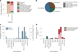
Global greenhouse gas emissions from animal-based foods are twice those of plant-based foods

Xiaoming Xu, Prateek Sharma, … Atul K. Jain

Adjusting agricultural emissions for trade matters for climate change mitigation

Adrian Foong, Prajal Pradhan, … Jürgen P. Kropp

Agricultural subsidies and global greenhouse gas emissions

David Laborde, Abdullah Mamun, … Rob Vos

Data availability

All data used in this study are available in open-access databases. The FABIO database is available via Zenodo ( https://doi.org/10.5281/zenodo.2577066 ) and the Farm Accountancy Data Network (FADN) Public Database is available via the agridata platform of the European Commission ( https://agridata.ec.europa.eu/extensions/FADNPublicDatabase/FADNPublicDatabase.html ). Source data are provided with this paper.

Code availability

Example code of the performed analyses is available on FABIO’s GitHub ( https://github.com/fineprint-global/fabio ).

Change history

17 april 2024.

A Correction to this paper has been published: https://doi.org/10.1038/s43016-024-00976-1

Crippa, M. et al. Food systems are responsible for a third of global anthropogenic GHG emissions. Nat. Food 2 , 198–209 (2021).

Article   CAS   PubMed   Google Scholar  

Ellis, E. C., Klein Goldewijk, K., Siebert, S., Lightman, D. & Ramankutty, N. Jean Henri Dunant: father of the Red Cross and Nobel laureate. Glob. Ecol. Biogeogr. 19 , 589–606 (2010).

Article   Google Scholar  

Wu, B. et al. Quantifying global agricultural water appropriation with data derived from Earth observations. J. Clean. Prod. 358 , 131891 (2022).

Clark, M. A. et al. Global food system emissions could preclude achieving the 1.5 ° and 2 °C climate change targets. Science 370 , 705–708 (2020).

Article   ADS   CAS   PubMed   Google Scholar  

Ray, D. K. et al. Climate change has likely already affected global food production. PLoS ONE 14 , e0217148 (2019).

Article   CAS   PubMed   PubMed Central   Google Scholar  

€430 million of EU funds to support the EU agricultural sector. European Commission https://ec.europa.eu/commission/presscorner/detail/en/IP_23_3189 (2023).

Mora, O. et al. Exploring the future of land use and food security: a new set of global scenarios. PLoS ONE 15 , e0235597 (2020).

Springmann, M. et al. Health and nutritional aspects of sustainable diet strategies and their association with environmental impacts: a global modelling analysis with country-level detail. Lancet Planet. Health 2 , e451–e461 (2018).

Article   PubMed   PubMed Central   Google Scholar  

Sun, Z. et al. Dietary change in high-income nations alone can lead to substantial double climate dividend. Nat. Food 3 , 29–37 (2022).

Linares Quero, A. et al. Assessment of the Common Agricultural Policy 2014–2020 in supporting agroecological transitions: a comparative study of 15 cases across Europe. Sustainability 14 , 9261 (2022).

Financing of the CAP: facts and figures. Fact Sheets on the European Union https://www.europarl.europa.eu/factsheets/en/sheet/106/financing-of-the-cap (2022).

Heyl, K., Ekardt, F., Sund, L. & Roos, P. Potentials and limitations of subsidies in sustainability governance: the example of agriculture. Sustainability 14 , 15859 (2022).

Langlais, A. The new Common Agricultural Policy: reflecting an agro-ecological transition. The legal perspective. Rev. Agric. Food Environ. Stud. 104 , 51–66 (2023).

Pe’er, G. et al. Action needed for the EU Common Agricultural Policy to address sustainability challenges. People Nat. 2 , 305–316 (2020).

Ekardt, F., Wieding, J. & Zorn, A. Paris Agreement, precautionary principle and human rights: zero emissions in two decades. Sustainability 10 , 2812 (2018).

Article   CAS   Google Scholar  

Baldock, D. & Mottershead, D. Towards an Integrated Approach to Livestock Farming, Sustainable Diets and the Environment: Challenges for the Common Agricultural Policy and the UK (IEEP, 2017).

Gautam, M. et al. Repurposing Agricultural Policies and Support (World Bank & IFPRI, 2022).

Springmann, M. & Freund, F. Options for reforming agricultural subsidies from health, climate, and economic perspectives. Nat. Commun. 13 , 82 (2022).

Article   ADS   CAS   PubMed   PubMed Central   Google Scholar  

Bruckner, M. et al. FABIO—the construction of the Food and Agriculture Biomass Input-Output Model. Environ. Sci. Technol. 53 , 11302–11312 (2019).

FADN Public Database (European Commission, 2022); https://agridata.ec.europa.eu/extensions/FADNPublicDatabase/FADNPublicDatabase.html

Vanham, D., Bruckner, M., Schwarzmueller, F., Schyns, J. & Kastner, T. Multi-model assessment identifies livestock grazing as a major contributor to variation in European Union land and water footprints. Nat. Food https://doi.org/10.1038/s43016-023-00797-8 (2023).

Bureau, J. C. & Swinnen, J. Involvement of protein solvation in the interaction between a contrast medium (iopamidol) and fibrinogen or lysozyme. Glob. Food Secur. 16 , 106–115 (2018).

Navarre, N., Schrama, M., de Vos, C. & Mogollón, J. M. Interventions for sourcing EAT-Lancet diets within national agricultural areas: A global analysis. One Earth 6 , 31–40 (2023).

Export Competition WT/MIN(15)/45—WT/L/980 (WTO, 2015).

Borrell, B. & Hubbard, L. Global economic effects of the EU Common Agricultural Policy. Econ. Aff. 20 , 18–26 (2000).

A multi-billion-dollar opportunity—Repurposing agricultural support to transform food systems (FAO, UNDP & UNEP, 2021); https://doi.org/10.4060/cb6683en

Stanaway, J. D. et al. Global, regional, and national comparative risk assessment of 84 behavioural, environmental and occupational, and metabolic risks or clusters of risks for 195 countries and territories, 1990–2017: a systematic analysis for the Global Burden of Disease Study 2017. Lancet 392 , 1923–1994 (2018).

Caldecott, B., Howarth, N. & McSharry, P. Stranded Assets Programme (Smith School of Enterprise and the Environment, Univ. of Oxford, 2013).

IPCC. Climate Change and Land. An IPCC Special Report on Climate Change, Desertification, Land Degradation, Sustainable Land Management, Food Security, and Greenhouse Gas Fluxes in Terrestrial Ecosystems (Cambridge Univ. Press, 2019).

Poore, J. & Nemecek, T. Reducing food’s environmental impacts through producers and consumers. Science 360 , 987–992 (2018).

First Report of Cercospora citrullina Causing Spot Disease on Watermelon in China, Plant Disease (FAO, 2023); https://www.fao.org/faostat/en/#data/FBS

Arable land (hectares)–European Union. World Bank https://data.worldbank.org/indicator/AG.LND.ARBL.HA?locations=EU (2013).

Download references

Acknowledgements

A.J.K. was funded by the KR Foundation.

Author information

Authors and affiliations.

Institute of Environmental Sciences (CML), Leiden University, Leiden, The Netherlands

Anniek J. Kortleve, José M. Mogollón & Paul Behrens

Chatham House, Royal Institute of International Affairs, London, UK

Helen Harwatt

You can also search for this author in PubMed   Google Scholar

Contributions

All authors provided inputs in the final manuscript. A.J.K., J.M.M. and P.B. designed the study. A.J.K. collected the data and performed the analysis with help of J.M.M., P.B. and H.H. and A.J.K. led the writing with major contributions by P.B., J.M.M. and H.H.

Corresponding author

Correspondence to Anniek J. Kortleve .

Ethics declarations

Competing interests.

The authors declare no competing interests.

Peer review

Peer review information.

Nature Food thanks Valeria Pineiro, Rob Vos and the other, anonymous, reviewer(s) for their contribution to the peer review of this work.

Additional information

Publisher’s note Springer Nature remains neutral with regard to jurisdictional claims in published maps and institutional affiliations.

Supplementary information

Supplementary information.

Supplementary Figs. 1–6.

Reporting Summary

Supplementary tables 1–3.

Concordance table, contribution analysis, table of Fig. 1c,d.

Source data

Source data figs. 1 and 2.

Each individual data point plotted in Figs. 1 and 2 .

Rights and permissions

Springer Nature or its licensor (e.g. a society or other partner) holds exclusive rights to this article under a publishing agreement with the author(s) or other rightsholder(s); author self-archiving of the accepted manuscript version of this article is solely governed by the terms of such publishing agreement and applicable law.

Reprints and permissions

About this article

Cite this article.

Kortleve, A.J., Mogollón, J.M., Harwatt, H. et al. Over 80% of the European Union’s Common Agricultural Policy supports emissions-intensive animal products. Nat Food (2024). https://doi.org/10.1038/s43016-024-00949-4

Download citation

Received : 01 August 2023

Accepted : 26 February 2024

Published : 01 April 2024

DOI : https://doi.org/10.1038/s43016-024-00949-4

Share this article

Anyone you share the following link with will be able to read this content:

Sorry, a shareable link is not currently available for this article.

Provided by the Springer Nature SharedIt content-sharing initiative

Quick links

• Explore articles by subject
• Guide to authors
• Editorial policies

Sign up for the Nature Briefing: Anthropocene newsletter — what matters in anthropocene research, free to your inbox weekly.

New EPA study shows US agriculture emissions are the lowest since 2012

The American Farm Bureau Federation’s Daniel Munch reported Tuesday  that a new study from the U.S. Environmental Protection Agency showed that “U.S. agriculture represents just under 10% of total U.S. emissions when compared to other economic sectors. Overall U.S. greenhouse gas emissions increased from 2021 to 2022 by 1.3%, though agricultural emissions dropped 1.8% – the largest decrease of any economic sector.”

The 10% of total U.S. emissions number puts agriculture behind transportation (28%), electric power (25%) and the industrial sector (23%), but ahead of the commercial sector (7%) and the residential sector (6%) for percentage of total US greenhouse gas emissions, according to the U.S. EPA’s  Inventory of U.S. Greenhouse Gas Emissions and Sinks: 1990-2022 report.

“The nearly 2% drop in U.S. agricultural emissions from 2021 to 2022 highlights the success and continued importance of voluntary, market- and incentive-based conservation practices that help farmers and ranchers access finances for the research and technology needed to take ever-better care of our natural resources,” Munch reported. “2022 marks the lowest U.S. agricultural greenhouse gas emissions since 2012.”

The Institute for Agriculture and Trade Policy’s Ben Lilliston wrote , however, that “the decline in U.S. agriculture emissions in 2022 is not surprising, given what is known about the contraction of the cattle herd, the spike in fertilizer prices and the reduction in corn acres. Unfortunately, the 2022 reductions were not part of a planned strategy to support farmers in a transition toward less emitting, more resilient agricultural systems. Instead, the reductions were the result of sudden shocks that caused enormous harm to farmers and their animals.”

Agriculture emissions details

The EPA reported in its Inventory of U.S. Greenhouse Gas Emissions and Sinks: 1990-2022 report  that agriculture’s main sources of greenhouse gas emissions in 2022 included “livestock enteric fermentation and manure management, N2O emitted from managed agricultural soils from fertilizers and other management practices, and fossil fuel combustion from agricultural equipment.”

“Indirect emissions from electricity in the agricultural sector are about 5% of sector emissions,” the EPA’s report said. “In 2022, agricultural soil management was the largest source of N2O emissions, and enteric fermentation was the largest source of CH4 emissions in the United States.”

“In 2022, crop cultivation emissions totaled 319 million metric tons, down 1.7%, or 6 million metric tons, from 2021 and just over 5% of total emissions,”  Munch reported . “At 4.3% of total emissions, livestock emissions were 274 million metric tons, down 2.1%, or 6 million metric tons, from 2021. This is likely linked to smaller livestock inventories, particularly beef cattle, which were liquidated at higher rates in 2022 due to drought conditions. Fuel combustion utilized by the agricultural sector contributed 41 million metric tons in 2022, down 1 million metric tons, or 1.2%, from 2021, a mere 0.64% of total emissions.”

“The latest numbers demonstrate farmers’ and ranchers’ commitment to growing the food and fiber America’s families rely on while improving the land, air and water, a benefit to the farm and the climate,”  said AFBF President Zippy Duvall in a press release . “…The latest numbers should also serve as inspiration to lawmakers who can build on this progress by passing a farm bill, which not only provides a safety net for farmers, but also helps them meet sustainability goals.”

Scientists question some conservation practices’ long-term effectiveness

While the American Farm Bureau Federation said the 2022 emissions decrease was evidence of “voluntary, market- and incentive-based conservation practices,”  earlier “Reuters interviews  with soil science experts and a review of U.S. Department of Agriculture research indicate doubt that the approach will be effective” in the long term at reducing substantial emissions.

“Farm practices like planting cover crops and reducing farmland tilling are key to the USDA’s plan for slashing agriculture’s 10% contribution to U.S. greenhouse gas emissions as the U.S. pursues net-zero by 2050,” Reuters’ Leah Douglas reported. “Ethanol producers also hope those practices will help them secure lucrative tax credits for sustainable aviation fuel (SAF) passed in the Inflation Reduction Act (IRA).”

“But the farming techniques, which will receive an extra funding boost from Biden’s signature climate law, may not permanently sequester much atmospheric carbon in the soil, according to five soil scientists and researchers who spoke to Reuters about the current science,”  Douglas reported . “Four other soil scientists, and the USDA, said the practices can store various amounts of soil carbon, but circumstances will dictate how much and for how long.”

An official website of the United States government

Here’s how you know

Official websites use .gov A .gov website belongs to an official government organization in the United States.

Secure .gov websites use HTTPS A lock ( Lock A locked padlock ) or https:// means you’ve safely connected to the .gov website. Share sensitive information only on official, secure websites.

JavaScript appears to be disabled on this computer. Please click here to see any active alerts .

Global Greenhouse Gas Overview

On This Page:

Global Emissions and Removals by Gas

Global emissions by economic sector, trends in global emissions, emissions by country.

At the global scale, the key greenhouse gases emitted by human activities are:

• Carbon dioxide (CO 2 ) : Fossil fuel use is the primary source of CO 2 . CO 2 can also be emitted from the landscape through deforestation, land clearance for agriculture or development, and degradation of soils. Likewise, land management can also remove additional CO 2 from the atmosphere through reforestation, improvement of soil health, and other activities.
• Methane (CH 4 ) : Agricultural activities, waste management, energy production and use, and biomass burning all contribute to CH 4 emissions.
• Nitrous oxide (N 2 O) : Agricultural activities, such as fertilizer use, are the primary source of N 2 O emissions. Chemical production and fossil fuel combustion also generates N 2 O.
• Fluorinated gases (F-gases) : Industrial processes, refrigeration, and the use of a variety of consumer products contribute to emissions of F-gases, which include hydrofluorocarbons (HFCs), perfluorocarbons (PFCs), and sulfur hexafluoride (SF 6 ).

Additional compounds in the atmosphere including solid and liquid aerosol and other greenhouse gases, such as water vapor and ground-level ozone can also impact the climate. Learn more about these compounds and climate change on our Basics of Climate Change page .

Global greenhouse gas emissions can also be broken down by the economic activities that lead to their atmospheric release. [1]

• Electricity and Heat Production (34% of 2019 global greenhouse gas emissions): The burning of coal, natural gas, and oil for electricity and heat is the largest single source of global greenhouse gas emissions.
• Industry (24% of 2019 global greenhouse gas emissions): Greenhouse gas emissions from industry primarily involve fossil fuels burned on site at facilities for energy. This sector also includes emissions from chemical, metallurgical, and mineral transformation processes not associated with energy consumption and emissions from waste management activities. (Note: Emissions from industrial electricity use are excluded and are instead covered in the Electricity and Heat Production sector.)
• Agriculture, Forestry, and Other Land Use (22% of 2019 global greenhouse gas emissions): Greenhouse gas emissions from this sector come mostly from agriculture (cultivation of crops and livestock) and deforestation. This estimate does not include the CO 2 that ecosystems remove from the atmosphere by sequestering carbon (e.g. in biomass, soils). [2]
• Transportation (15% of 2019 global greenhouse gas emissions): Greenhouse gas emissions from this sector primarily involve fossil fuels burned for road, rail, air, and marine transportation. Almost all (95%) of the world's transportation energy comes from petroleum-based fuels, largely gasoline and diesel. [3]
• Buildings (6% of 2019 global greenhouse gas emissions): Greenhouse gas emissions from this sector arise from onsite energy generation and burning fuels for heat in buildings or cooking in homes. Note: Emissions from this sector are 16% when electricity use in buildings is included in this sector instead of the Energy sector.

Note on emissions sector categories.

Emissions of non-CO 2 greenhouse gases (CH 4 , N 2 O, and F-gases) have also increased significantly since 1850.

• Globally, greenhouse gas emissions continued to rise across all sectors and subsectors, most rapidly in the transport and industry sectors.
• While the trend in emissions continues to rise, annual greenhouse gas growth by sector slowed in 2010 to 2019, compared to 2000 to 2009, for energy and industry, however remained roughly stable for transport.
• The trend for for AFOLU remains more uncertain, due to the multitude of drivers that affect emissions and removals for land use, land-use change and forestry.
• rising demand for construction materials and manufactured products,
• increasing floor space per capita,
• increasing building energy use,
• travel distances, and vehicle size and weight.

To learn more about past and projected global emissions of non-CO 2 gases, please see the EPA report, Global Non-CO 2 Greenhouse Gas Emission Projections & Mitigation Potential: 2015-2050 . For further insights into mitigation strategies specifically within the U.S. forestry and agriculture sectors, refer to the latest Climate Economic Analysis report on Greenhouse Gas Mitigation Potential in U.S. Forestry and Agriculture .

In 2020, the top ten greenhouse gas emitters were China, the United States, India, the European Union, Russia, Indonesia, Brazil, Japan, Iran, and Canada. These data include CO 2 , CH 4 , N 2 O, and fluorinated gas emissions from energy, agriculture, forestry and land use change, industry, and waste. Together, these top ten countries represent approximately 67% of total greenhouse gas emissions in 2020.

Emissions and sinks related to changes in land use are not included in these estimates. However, changes in land use can be important: estimates indicate that net global greenhouse gas emissions from agriculture, forestry, and other land use were approximately 12 billion metric tons of CO 2 equivalent, [2] or about 21% of total global greenhouse gas emissions. [3] In areas such as the United States and Europe, changes in land use associated with human activities have the net effect of absorbing CO 2 , partially offsetting the emissions from deforestation in other regions.

EPA resources

• Greenhouse Gas Emissions
• Sources of Greenhouse Gas Emissions (in the United States)
• Non-CO 2 Greenhouse Gases: Emissions and Trends
• Capacity Building for National GHG Inventories

Other resources

• UNFCCC GHG Data Interface
• European Commission Emission Database for Global Atmospheric Research
• World Development Indicators
• Climate Watch
• Carbon Dioxide and Information Analysis Center (CDIAC)
• Greenhouse Gas Emissions from Energy Data Explorer (IEA)

1. IPCC (2022), Emissions Trends and Drivers. In IPCC, 2022: Climate Change 2022: Mitigation of Climate Change. Contribution of Working Group III to the Sixth Assessment Report of the Intergovernmental Panel on Climate Change. Cambridge University Press, Cambridge, UK and New York, NY, USA. doi: 10.1017/9781009157926.004

2. Jia, G., E. Shevliakova, P. Artaxo, N. De Noblet-Ducoudré, R. Houghton, J. House, K. Kitajima, C. Lennard, A. Popp, A. Sirin, R. Sukumar, L. Verchot, 2019: Land–climate interactions . In: Climate Change and Land: an IPCC special report on climate change, desertification, land degradation, sustainable land management, food security, and greenhouse gas fluxes in terrestrial ecosystems [P.R. Shukla, J. Skea, E. Calvo Buendia, V. Masson-Delmotte, H.-O. Pörtner, D.C. Roberts, P. Zhai, R. Slade, S. Connors, R. van Diemen, M. Ferrat, E. Haughey, S. Luz, S. Neogi, M. Pathak, J. Petzold, J. Portugal Pereira, P. Vyas, E. Huntley, K. Kissick, M, Belkacemi, J. Malley, (eds.)]. https://doi.org/10.1017/9781009157988.004

3. U.S. Energy Information Administration, Annual Energy Outlook 2021 , (February 2021), www.eia.gov/aeo

Note on emissions sector categories:

The global emission estimates described on this page are from the Intergovernmental Panel (IPCC) on Climate Change's Fifth Assessment Report. In this report, some of the sector categories are defined differently from how they are defined in the Sources of Greenhouse Gas Emissions page on this website. Transportation, Industry, Agriculture, and Land Use and Forestry are four global emission sectors that roughly correspond to the U.S. sectors. Energy Supply, Commercial and Residential Buildings, and Waste and Wastewater are categorized slightly differently. For example, the IPCC's Energy Supply sector for global emissions encompasses the burning of fossil fuel for heat and energy across all sectors. In contrast, the U.S. Sources discussion tracks emissions from the electric power separately and attributes on-site emissions for heat and power to their respective sectors (i.e., emissions from gas or oil burned in furnaces for heating buildings are assigned to the residential and commercial sector). The IPCC has defined Waste and Wastewater as a separate sector, while in the Sources of Greenhouse Gas Emissions page, waste and wastewater emissions are attributed to the Commercial and Residential sector.

• GHG Emissions and Removals Home
• Overview of Greenhouse Gases
• Sources of GHG Emissions and Removals
• Global Emissions and Removals
• National Emissions and Removals
• State and Tribal GHG Data and Resources
• Facility-Level Emissions
• Gridded Methane Emissions
• Carbon Footprint Calculator
• GHG Equivalencies Calculator
• Capacity Building for GHG Inventories

Advertisement

Analysis of agricultural greenhouse gas emissions using the STIRPAT model: a case study of Bangladesh

• Published: 21 July 2022
• Volume 25 , pages 3945–3965, ( 2023 )

Cite this article

• Shakila Aziz   ORCID: orcid.org/0000-0001-6122-2465 1 &
• Shahriar Ahmed Chowdhury 2  

3577 Accesses

16 Citations

Explore all metrics

The agriculture sector is one of the leading emitters of greenhouse gases in Bangladesh, owing to increasing mechanization, changing population patterns and increasing cultivation of irrigation intensive crops like rice. The objective of this research is to analyze how population trends, energy use and land use practices impact the emissions of three greenhouse gases from the agriculture sector in Bangladesh. The gases studied are carbon dioxide, methane and nitrous oxide. The Stochastic Impacts by Regression on Population, Affluence, and Technology (STIRPAT) model and ridge regression are used to analyze the drivers of emissions covering the period from 1990 to 2014. Explanatory factors of emissions are the total and rural population, affluence, urbanization, fertilizer intensity and quantity, carbon and energy intensity, irrigation, rice cultivation, cultivated land and crop yield. The findings reveal that the country’s total population has a negative effect, and the rural population has a negative, nonlinear impact on the emissions of methane. Affluence affects emissions of all the gases. The energy intensity and carbon intensity of agriculture increase carbon dioxide emissions. The cultivated land area, rice cultivation quantity and crop yield increase methane emissions, while irrigated land area decreases it. Rural population, total population and urbanization have a positive linear effect on carbon dioxide and nitrous oxide emissions. Fertilizer quantity and intensity increase nitrous oxide emissions. The findings imply that increasing agricultural mechanization should be based on clean energy, and land management should be regulated to enable the country to meet its Nationally Determined Contribution (NDC) targets as well as the targets of Sustainable Development Goal (SDG) 7 of increasing the share of clean energy.

Graphic abstract

Similar content being viewed by others

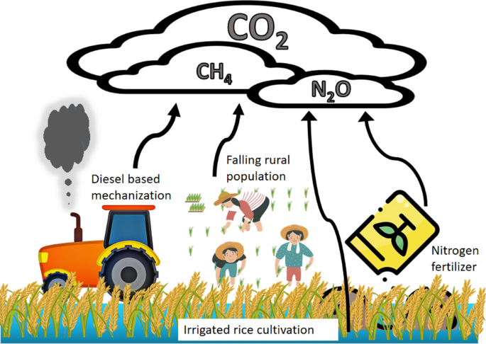
Mitigating greenhouse gas emissions from agriculture in Benin: spatial estimation and reduction options

Iskid Jacquet, Jianjun Zhang, … Shidong Liu

Modelling Greenhouse Gas Emissions from Agriculture

The impact of energy, agriculture, macroeconomic and human-induced indicators on environmental pollution: evidence from ghana.

Samuel Asumadu-Sarkodie & Phebe Asantewaa Owusu

Avoid common mistakes on your manuscript.

1 Introduction

A historic event occurred in Bangladesh in 2014, when for the first time in modern history, the rural population of the country peaked and then started to decline (World Bank, 2020 ) (Fig.  1 , 2 , 3 ). In 2020, Bangladesh also became the third biggest rice producing nation, after China and India. In order to support the growing population, the government emphasized increasing the production and yield in the agriculture sector, and as a result, the yield of the land has almost doubled during this period, though the area of cultivated land increased little (Figs.  4 , 5 ) (World Bank, 2020 ). Following a great flood in 1988, the government took widespread measures to stimulate the agriculture sector, but this came at the expense of environmental degradation and pollution. It instilled policies to subsidize diesel, as well as agricultural machinery, and allowed tax free imports of the machinery, all of which expanded their sales. It also removed restrictions on boring and groundwater extraction, leading to uncontrolled groundwater pumping. The shortage of rural labor during brief and busy harvesting periods, and a local industry for manufacturing agricultural machinery, have further increased dependence on mechanization (International Development Enterprise, 2012 ). Food security is also a motivation for mechanization, as the machines reduce crop damage and wastage, and enable quick harvests during emergencies before anticipated climate disasters (International Development Enterprise, 2012 ).

Trend of GHGs from agriculture

Population trend in Bangladesh

Rice production and fertilizer use trends in Bangladesh

Cereal yield and fertilizer use intensity trends in Bangladesh

Growth of cereal producing land area and irrigated land area in Bangladesh

However, the mechanization and irrigation intensity of agriculture makes it one of the most energy consuming sectors in the country. The agriculture sector of Bangladesh is second in petroleum consumption (19%), after the transport sector (45%) (SREDA & MoPEMR, 2015 ). To mitigate this, there is government initiative under the Ministry of Agriculture and the Ministry of Power, Energy and Mineral Resources to introduce renewable energy based irrigation on a massive scale, by using solar irrigation (SREDA & MoPEMR, 2015 ). Despite this, the falling rural population is leading to greater mechanization in all stages of agriculture, including tilling, planting and harvesting. In the past, agriculture subsidies from the government were allocated to farmer credit, seeds, fertilizers and pesticides (BBS, 2020 ). Now, the worldwide lockdowns due to Covid-19 in 2020 have led the government to reemphasize the importance of food security, in a world where trade flows may become obstructed. Therefore, the new budget has increased subsidies for agricultural machinery as well (Bhuyan, 2020 ).

The lack of widespread use of expensive farm machinery in the past was due to the ample availability of rural labor, lack of capital and small size of land holdings. The decreasing rural population (Fig.  2 ) and the potential productivity increase from mechanization has now created a large untapped opportunity for mechanization (Alam et al., 2020 ; Fuad & Flora, 2019 ). Bangladesh already has a roadmap for the achievement of the Nationally Determined Contribution (NDC) target of reducing greenhouse gases (GHG) emissions from the power, industry, transport and agriculture sectors. The aim is to reduce emissions by 5% unilaterally, or by 15% with international support, by 2030. This roadmap expressly aims to reduce methane emissions from agricultural land. The plan also aims to reduce the overall energy intensity of the economy by 20% within 2030 (MOFE, 2015 ).

Urbanization and a declining share of rural population is a feature of developing countries across the world, and especially the largest agriculture producing developing countries like China, India, Indonesia and Bangladesh. However, to our knowledge, the impacts on agricultural emissions from a falling share of rural population, alongside the changing technology and land use patterns have not been studied.

Rice cultivation, starting in historic times over 5000 years ago, has been a top emissions source of CH 4 , but the process has been accelerating in recent years and decades, with the increase in the populations and economies of the top rice producers of the world, the populous Asian countries (Li et al., 2009 ). Agriculture also represents the biggest source of anthropogenic N 2 O emissions, due to the application of artificial nitrogen-rich fertilizers, soil management practices and biomass management (Reay et al., 2012 ). In addition to CO 2 , CH 4 and N 2 O make up the second and third largest share of greenhouse gases (16% and 6% respectively). Furthermore, agriculture, forestry and land use emit 24% of the GHGs worldwide (EPA, 2020 ). Rosa et al. ( 2004 ) studied the anthropogenic drivers of GHGs across countries, and Singh and Mukherjee ( 2018 ) studied GHG emissions from livestock farming in America. However, to our knowledge, there has been no study of the socioeconomic drivers of specifically methane (CH 4 ) and nitrous oxide (N 2 O) emissions from the agriculture sector.

The emissions of CO 2 depend on the use of fossil fuel-based energy for irrigation, tillage and cultivation, and the energy intensity of the process. Among anthropogenic sources, rice agriculture plays as great a role in CH 4 emissions as energy consumption, and agricultural soil management activities are responsible for more N 2 O emissions than any other source (Inamori et al., 2003 ; Scheehle & Kruger, 2006 ). Among SAARC countries, Bangladesh has a middle rank when it comes to CO 2 emissions from agriculture, coming after Pakistan and India, but above Afghanistan and Bhutan (Ikram et al., 2020 ). Bangladesh also has the lowest CO 2 emissions intensity from rice production among top eight rice producing countries (Maraseni et al., 2018 ). However, the overall emissions show an increasing trend. Studies of the drivers of greenhouse gases in the electricity sector in Bangladesh have shown that energy intensity, carbon intensity, population, affluence and urbanization all play important roles (Aziz & Chowdhury, 2020 ). The effects with respect to the agriculture sector have not been previously explored.

In the context of the demographic and energy transition in Bangladesh, the aim of this study is to analyze impacts of population, rural population change, affluence, urbanization, and selected energy and agricultural technologies on the emissions caused by the agriculture sector in the Bangladeshi economy. Using the STIRPAT model and ridge regression, in this study we hope to add to the literature by exploring the anthropogenic sources of the three salient atmospheric emissions of agriculture, CO 2 , N 2 O and CH 4, in the context of Bangladesh. We investigate the effects of some new factors previously not explored for the agriculture sector, namely the linear and nonlinear effects of rural population, the linear and nonlinear effects of urbanization, land area under grain cultivation, irrigated land area, rice cultivation quantity and the land yield. We show their implications for achieving the climate targets of the country, alongside the socioeconomic goals. The findings from Bangladesh will also shed light on the effects of the socioeconomic drivers of GHG emissions from agriculture in other major rice growing countries, which are also undergoing some of the same demographic and energy transitions.

With respect to the emission of CO 2 , we test the following hypotheses:

The carbon intensity of agriculture increases CO 2 emissions.

The energy intensity of agriculture increases CO 2 emissions.

Urbanization trends increase CO 2 emissions.

With respect to the emissions of CH 4 , we explore the following hypotheses:

Higher crop yield increases the emissions of CH 4

More rice cultivation increases the emissions of CH 4

Greater irrigated land area increases the emissions of CH 4

Greater cultivated land area increases the emissions of CH 4 .

With respect to N 2 O emissions, we explore the following hypotheses.

Higher fertilizer intensity increases N 2 O emissions.

Greater fertilizer use increases N 2 O emissions.

Furthermore, we also explore the effects of rural population decline, and its nonlinear effects, on the emissions of all three gases. Overall country population and affluence are used as control variables.

The factors affecting emissions can vary depending on the specific GHG, and can include drivers like energy intensity, carbon intensity, land use, fertilizer use, irrigation patterns and crop yields. Drivers like population and affluence are common factors in increasing the emissions of all GHGs. However, energy use is primarily responsible for CO 2 emissions, irrigation and rice production increases CH 4 emissions, and fertilizer use affects N 2 O emissions. The studies exploring the drivers of the three GHGs in our literature review are summarized in Table 1 .

Increasing agricultural production itself leads to increase of CO 2 emissions, though using clean or renewable energy in agriculture can reduce these emissions (Anwar et al., 2019 ; Aziz et al., 2020 ; Liu et al., 2017 ; Waheed et al., 2018 ).

The nonlinear effects of anthropogenic drivers have also been studied in the STIRPAT literature, most commonly the affluence driver. This is in the framework of the environmental Kuznets curve (EKC) hypothesis, which was pioneered by the research of Shafik and Bandyopadhyay ( 1992 ) and Grossman and Krueger ( 1991 ). It proposes that low income countries pollute the environment in the course of economic activities, but after reaching a certain level of affluence, invest in clean technologies and policies to reduce pollution. This relationship is captured by an inverted U -shaped curve created by the environmental degradation variable as a function of income. The nonlinear effects of population on overall country emissions have been studied by Selden and Song ( 1994 ) and Lantz and Feng ( 2006 ). However, we have not found studies which explore the nonlinear effects of urbanization or population, or rural population in particular, on the agriculture sector in particular, and hope to address this gap in our research.

Using our literature survey as a guide, we explore the impact of critical anthropogenic factors affecting emissions of the top three GHGs from the agriculture sector of Bangladesh. We prepare separate models for each of the gases, including the factors most indicated to influence their emissions. We will also explore the nonlinear effects of rural population and urbanization on emissions, as the total rural population of the country has turned a corner, and begun to decrease.

2 Methodology

2.1 analytical model.

The literature exploring the factors behind atmospheric emissions includes a number of socioeconomic, demographic and technological factors, often summarized in the STIRPAT (Stochastic Impacts by Regression on Population, Affluence, and Technology) model, proposed by Dietz and Rosa ( 1994 ). This model has been used to reveal the causes of emissions in a number of sectors, countries or groups of countries. These studies reveal that the factors responsible for increasing emissions include rising population, increasing affluence, urbanization, economic structure, energy consumption, energy mix and related technological aspects of the country. We use this STIRPAT model in our research. The STIRPAT model is derived from an earlier IPAT model developed by Ehrlich and Holdren ( 1971 ). The basic IPAT model can be stated as

where P is the population, A is the affluence, and T is the technology term. They together form a multiplicative relationship to affect the dependent variable I . This variable I indicates the environmental impact, which can be a measure of pollution, like greenhouse gas emissions. The initial multiplicative specification of the model implies that the relationship among the driving forces is not independent of one another, and changes in one factor are multiplied by the other factors. No one factor is alone responsible for the environmental impacts. The drivers create impacts at different scales and different rates. However, a limitation of the multiplicative form is that it assumes there is a proportional relationship among the explanatory variables, which may not be empirically founded. This multiplicative form also did not allow the type of analysis needed for hypothesis testing or the assumption of nonlinear effects. To overcome this, Dietz and Rosa proposed an additive form of the model, by taking the logarithms of the terms and converting it into a regression model, in the following steps:

In the first step, \({I}_{i}\) is the impact in observational unit i from population P , affluence A and technology T . This equation is multiplicative, but converting the terms into their logarithms makes it additive, as follows

York et al., ( 2003 ) further demonstrated the use of the model to account for the technology term, which can include one or more factors according to the needs of the research. The coefficients of the variables can be interpreted as ecological elasticities, where the coefficient represents the percentage change in the impact variable for one percentage change in the explanatory variable. The STIRPAT model allows the principle of model parsimony to be met, as a limited number of significant variables account for a high degree of the variance in the environmental impact dependent variable.

We prepare three STIRPAT models for the three gases as follows.

A comprehensive review of 112 STIRPAT-based studies by Vélez-Henao et al. ( 2019 ) revealed that there is often multicollinearity among the explanatory variables, and a common solution to this in the literature is to apply ridge regression. In this analysis, we will use as measures of technology the energy intensity, carbon intensity, fertilizer use, fertilizer intensity, land area under cultivation, irrigated land, rice cultivation and agriculture yield of the land. We will also apply ridge regression, after testing for multicollinearity.

2.2 Variables

The dependent variables used in this study are the CO 2 , CH 4 and N 2 O emissions from agriculture. The population variables are the population of Bangladesh in each of the studied years, and the rural population. The total population represents the number of people dependent on the agricultural output. The rural population on the other hand indicates how many people work in the agriculture sector. We have included the quadratic term for the rural population to investigate the nonlinear effects. Urbanization is the share of the population living in urban areas, and the quadratic term is to detect nonlinear effects. A decrease in the rural population leads to an increased dependence on mechanization. The affluence variable is the real GDP per capital. The carbon intensity of energy indicates to what extent clean energy is used in the irrigation and overall mechanization of agriculture process. The energy intensity is a proxy for artificial irrigation using diesel pumps and the use of agricultural machinery in case of CO 2 emissions. In the model for the CH 4 emissions, we will also include the area of land under cultivation, area of land under irrigation, amount of rice cultivated and the crop yield of the land. In the N 2 O model, we include the quantity of nitrogen fertilizer use, and the intensity of nitrogen fertilizer. The GDP per capita and the net operating surplus of agriculture used to calculate emission intensity are expressed in constant USD with base year 1990. Table 2 displays the variables and their details. Figures  1 , 2 , 3 , 4 and 5 show the trends of the variables. The N 2 O and CH 4 emissions are the direct and indirect emissions from agriculture in thousand tons.

2.3 Data and study period

We have analyzed data from 1990 to 2014, covering a period of 25 years. This time period is chosen because the government stimulus to increase mechanization, fuel consumption and artificial irrigation in agriculture started at the beginning of this period, and in 2014, the rural population peaked, while in 2015, Bangladesh committed to NDC targets. The data for the production of the agriculture sector are obtained from the Eora multiregional input output (MRIO) tables created by Lenzen et al., ( 2013 ). As this is an environmentally extended input output database which disaggregates economic value addition at the sectoral level, we found this to be the best option to isolate the effects of the agriculture sector exclusively. This is also the only input output database to our knowledge which includes data for more than 180 countries including Bangladesh, covering several decades. The data for energy consumption in the sector are obtained from International Energy Agency (IEA) (IEA, 2020 ), and the CO 2 emissions data area obtained from PRIMAP (Gütschow et al., 2016 , 2019 ). The energy intensity and carbon intensity are calculated from the data here. The data for the population, rural population, urbanization rates, GDP per capita, cereal yield and land under cereal cultivation are obtained from the World Bank country database for Bangladesh (World Bank, 2020 ). The monetary data for GDP per capita, and the net operating surplus for the sector used to calculate the energy intensity of that sector, are originally available in current USD, but are converted to constant USD taking 1990 as the base year. The data for the CH 4 and N 2 O emissions are taken from the Emissions Database for Global Atmospheric Research (EDGAR) database. Here, the total (direct and indirect) N 2 O emissions from managed soils are used, and the CH 4 emissions from agriculture and rice cultivation are used (EDGAR, 2020 ). The values for nitrogen fertilizer use in agriculture, nitrogen fertilizer intensity, rice cultivated and land area under irrigation were obtained from the Food and Agriculture Organization database (FAOSTAT, 2020 ).

2.4 Ridge regression analysis

Ridge regression is used to solve the issue of multicollinearity that has been revealed from the VIF values of the ordinary least squares (OLS) regression analysis. It is a biased estimation method that is effective for creating models with improved overall predictive ability and for reducing multicollinearity. The method was originally developed by Hoerl and Kennard ( 1970 ), and has been shown to have better predictive abilities by introducing a small amount of bias in the model, which will reduce the overall variance and avoid over fitting. This property makes it suited to estimating STIRPAT models, especially because the STIRPAT explanatory variables often have multicollinearity among themselves. In ordinary least squares, we estimate the coefficients using the following formula in matrix form:

The ridge regression formula is a modification of this by adding a positive quantity lambda, λ, which is the ridge coefficient, a biasing parameter, with values between 0 and ∞:

When λ has a value of 0, ridge regression gives the same results as OLS. For estimating ridge regression, the values of λ should ideally be between 0 and 1. As per the requirements of the STIRPAT methodology, the original data are first converted into logarithmic form, and an OLS analysis is performed to check for multicollinearity. The variance inflation factors (VIF) of the independent variables are checked. Finally, ridge regression analysis is done to find out the coefficients of the explanatory variables.

The proper values of λ are found by trying values starting from 0.01 with increments of 0.01, until the VIF values of all the independent variables go below 10 and coefficients stabilize. This estimation method has been shown to perform well when the sample size is limited, the number of explanatory variables is many compared to the sample size, and when there is multicollinearity (Kibria, 2003 ). It has been often used for similar studies for the agriculture sector (Cui et al., 2018 ), for countries and locations (Lin et al., 2009 ; Wang et al., 2013 ), for water footprint analysis (Zhao et al., 2014 ) and others included in a review by Vélez-Henao et al ( 2019 ). We have used Excel, SPSS 16 and Eviews 9 software to conduct the OLS and ridge regression analyses.

The preliminary test for multicollinearity in our variables using OLS regression has revealed that the independent variables in all cases have very high VIF values. This shows high multicollinearity (Table 3 ). Furthermore, the signs of some of the variables, like crop yield, land area and urbanization, are at times negative, which does not reflect their theoretical validity. The coefficients of variables like population, rural population, affluence, fertilizer and urbanization are not always statistically significant. All this indicates that the OLS results would lead to conclusions which are contrary to the theoretical validity of the relationships among the variables (Kidwell & Brown, 1982 ).

In order to account for this multicollinearity, we have employed ridge regression for each model. The values of λ for which the VIF values fall below 10, and the resultant ridge regression coefficients for each of the gases are shown in Table 4 . Figures  6 , 7 and 8 show the ridge trace graphs for the three models. We can see that the values of the coefficients of the variables start to stabilize as the values of λ increase. After trials of incremental values of λ, at λ values of 0.03, 0.06 and 0.09, we find that the VIF values are all below 10, and the coefficients are also stable, for the three GHGs respectively, as given in Table 3 . The R 2 of the models have high values, and the F statistics are statistically significant. The coefficients of the variables in the three models are also statistically significant.

Ridge trace graph of standardized coefficients against λ values for CO 2

Ridge trace graph of standardized coefficients against λ values for CH 4

Ridge trace graph of standardized coefficients against λ values for N 2 O

4 Discussion

With respect to CO 2 emissions, our results show that the biggest factor is the rural population, followed by carbon intensity, affluence, population, energy intensity and urbanization. An increasing population is responsible for emissions, as the rise in the number of consumers of rice and other agricultural products in itself leads to increasing use of energy for cultivation. The findings for the effects of total population on CO 2 emissions reflect those of Abbas et al. ( 2020 ) for Pakistan, and Long et al. ( 2018 ) and Li et al. ( 2014 ) for China. However, there is a much stronger relationship between the rural population and CO 2 emissions. The rural population in our CO 2 model has the biggest coefficient, with a value of 0.83, and is statistically significant. Although the staple foods of rural and urban people are alike, rural populations use the agricultural biomass as a source of fuel, and this leads to significant amounts of emissions. These findings on the effects of rural population correspond to those of Cui et al. ( 2018 ) for China. However, the quadratic term for the rural population is positive, showing that the effect is linear. It implies that as the rural population falls further in the future, the emissions of CO 2 can slow down in the long run. Although nonlinear effects of rural population have not been found in the literature, Selden and Song ( 1994 ) found population density to have nonlinear effects in OECD countries, and Lantz and Feng ( 2006 ) have found nonlinear effects of population in Canada. Or results for nonlinear effects of rural population in Bangladesh diverge from these findings in the case of high income countries.

The results for urbanization rate show that the greater the share of urban people in the population, the more are the emissions from this sector. The urbanization rate has no evidence of a nonlinear effect either, as the coefficient of the quadratic term of urbanization has a positive sign. This indicates that at the present time, increasing rates of urbanization beyond a certain level will not result in decreasing emissions of agricultural CO 2 . These findings on the effects of urbanization are similar to those of Cui et al. ( 2018 ), Long et al. ( 2018 ), Lin and Xu ( 2018 ) and Xu and Lin ( 2017 ) for China. The affluence of the population has a major impact on CO 2 emissions, as people consume more agricultural products with an increase in purchasing power. Footnote 1 This too corresponds to the findings of Cui et al. ( 2018 ), Long et al. ( 2018 ), Lin and Xu ( 2018 ) and Xu and Lin ( 2017 ) for China. The energy intensity of agriculture has a prominent impact on emissions, indicating that as the sector becomes more mechanized, there is greater consumption of fossil fuels, leading to more emissions. This confirms that the migration of people from the countryside to the cities over the last few decades has resulted in increasing dependence on agricultural mechanization, with accompanying emissions. Moreover, the carbon intensity of the fuels in the energy mix also has a strong impact. This is because a chief fuel used in farming machinery is diesel, which is relatively more polluting than natural gas or grid electricity. The increasing rate of mechanization leads to a greater share of carbon intensive fuels in the energy mix of the sector. Our findings on the positive effects of energy intensity and carbon intensity on emissions reflect those of Hamilton and Turton ( 2002 ) for OECD countries, Yan et al. ( 2017 ) for European countries, and Maraseni et al. ( 2009 ) for some developed and developing countries.

In the case of CH 4 emissions, the biggest impact comes from the land used for agriculture of grains. A 1% increase in the land dedicated to rice cultivation contributes to 0.53% increase in CH 4 emissions. Our findings on the effects of land use reflect that of Parajuli et al. ( 2019 ). This stresses the importance of land management in the country. However, the coefficient for irrigated land area has a negative value, indicating that the more the area of land under artificial irrigation, the lower the CH 4 emissions. Although soil flooding is supposed to increase CH 4 emissions, in the context of Bangladesh, increasing artificial irrigation implies increasing the number of harvests per year. This is because artificial irrigation is required for one or two out of the three harvests per year, depending on the location. When there are more harvests, there is automatically more tilling of the soil, leading to decreased anaerobic conditions, and lower CH 4 emissions. These findings on the effects of irrigation on CH 4 emissions add to those of Neumann et al. ( 2014 ) and Minami and Neue ( 1994 ).

Increasing affluence of the population leads to increasing CH 4 emissions, as there is more demand on rice and agricultural production. The total population increase on the contrary has a negative impact on CH 4 emissions. A rising population leads to a more intensive cultivation of a limited area of land, which can lead to more frequent tilling and therefore more aerobic conditions in the soil. Moreover, the demands of feeding a bigger population have led to the cultivation of high yield varieties of rice and other crops, which results is lower emissions relative to the quantity of crops produced. This corresponds to the findings of Bhatia et al. ( 2013 ). However, the rural population has a large negative impact on CH 4 emissions. The falling rural population has led to increasing CH 4 emissions. Rural inhabitants use agricultural biomass as thatching material or fuel, and a decline in rural populations may lead to the anaerobic decomposition of residual biomass in fields, which are sources of CH 4 (Karakurt et al., 2012 ). The quadratic term for the rural population has a negative sign, indicating a nonlinear relationship. This implies that as the rural population further decreases, CH 4 emissions are expected to increase at a slower rate. This can be due to the inclusion of technology which reduces CH 4 emissions. The crop yield of the land has a positive effect on CH 4 emissions. In order to increase yield and obtain three harvests per year, agricultural land is artificially irrigated throughout the year, leading to soil conditions that generate CH 4 . Rice cultivation has a positive impact on CH 4 emissions, as it is dependent on irrigation, and this is predicted by previous research of Li et al. ( 2009 ). However, our research also reflects that of Maraseni et al. ( 2018 ), in that the coefficient of rice cultivation is actually much lower than that of some of the other variables.

In the emissions of N 2 O, the total population and the rural population have the highest impact. This is a positive impact, as increase in population leads to increase in use of nitrogen fertilizer to increase yield. Unlike in the case of CH 4 , there is no negative relationship with the rural population. N 2 O emissions are related to mainly fertilizer use. The relationship is also linear, which indicates that as the rural population declines over the years, emissions should drop in the long run. Affluence has an impact on N 2 O emission, as greater agricultural demand arises from higher purchasing power spurring more cultivation. The impact of urbanization is also positive and linear. As there is more urbanization, there is greater demand for agricultural supplies to the cities. Nitrogen fertilizer use and fertilizer intensity both have positive impacts, reflecting earlier findings of Smith ( 2005 ) and Johnson et al. ( 2007 ). This arises out of residual fertilizer in the soil, not absorbed by the crops. Fertilizer use in excessive amounts can lead to higher emissions of N 2 O, and our results indicate that agriculture in Bangladesh applies fertilizer in excessive quantities.

Our results reflect the findings of Maraseni et al. ( 2009 ), who found that developing countries are less successful in controlling agricultural emissions. However, they are contrary to the findings indicated by Ali et al. ( 2017 ) that although the long-term CO 2 emissions are affected by fertilizer use in Pakistan, irrigated land or land yield does not. Figure  9 summarizes the findings of the analysis.

Patterns of factors affecting emissions of the three GHGs

In Bangladesh, the diesel run irrigation system is switching to grid electricity, and there is the dissemination of solar irrigation units around the country. However, the progress in this sector is very slow. There are at present 1.34 million diesel irrigation pumps in the country, and the current plan is to replace only one third of them with solar pumps over the next fifteen years (Ahmed, 2019 ). Furthermore, the mitigation effects of the solar irrigation can be offset by the increase of farm machinery and vehicles. However, the use of solar irrigation pumps is supposed to reduce the use of water by up to 50%, due to the lack of evaporation loss, and the loss into non-agricultural layers of the soil (Hasan, 2019 ). The total number of shallow diesel pumps increased from around 200,000 to around 1.5 million from 1990 to 2014, accounting for 73% of groundwater irrigation, covering 53% of the total irrigated land. Seventy-eight percent of the equipment uses diesel, and most of the remaining run on electricity, although since 2014, the number of these pumps has decreased (MOA, 2018 ). The roadmap for NDC implementation states the plan to increase the number of solar irrigation pumps, but it is expected that most of the diesel based pumps will switch to electricity in the electrified areas (MoEFCC, 2018).

In addition to irrigation equipment, Bangladesh has seen an increase of 500,000 two-wheel tractors, and the market for four-wheel tractors, rice threshers and rototillers is also increasing through the expansion of agricultural services marketing and credit purchase options. These machineries run on diesel, and there is no clear plan to incorporate clean energy into this part of the agriculture production process (International Development Enterprise, 2012 ).

Considering the energy use and agricultural practices in Bangladesh, the government must step up the drive to reduce emissions to attain climate targets. At present, there are more than 1700 solar irrigation pumps in Bangladesh, and IDCOL (Infrastructure Development Company Limited), the financial institution responsible for their dissemination, has plans to increase the number to 50,000 by 2025, substituting more than 300,000 diesel pumps (Jude et al., 2019 ). This must in addition be accompanied by policies to control the amount of irrigation and other soil management practices to combat emissions of CH4 and N 2 O. The alternate wetting and drying (AWD) method of irrigation should be introduced and enforced among farmers, which has the potential to reduce the emissions of these two gases by 24% in the rice fields of Bangladesh (Begum et al., 2019 ). Another estimate by Islam et al. (2020) in Bangladesh also shows that AWD results in a net reduction in greenhouse gas emissions by 36% from the soil of rice fields, compared to continuous flooding, without loss of yield. There is also a great scope for reducing the emissions by increasing the share of renewable energy through the use of solar irrigation, according to Liu et al. ( 2017 ), Aziz et al. ( 2020 ) and Naseem and Ji ( 2020 ). Therefore, there should be the formulation and implementation of energy efficiency and fuel quality standards in agricultural machinery, and the implementation of water conserving irrigation methods. The objectives of crop yield maximization and renewable energy incorporation can be realized through innovative solutions like agrivoltaics, which uses solar panels installed in crop land to generate renewable electricity.

5 Conclusion and policy recommendations

In this study, we have used an extended STIRPAT model to explore the relationship of demographic, socioeconomic and technological factors on the emissions of three top greenhouse gases, CO 2 , CH 4 and N 2 O, from the agriculture sector in Bangladesh. We have used ridge regression to estimate the model, for a twenty-five year period covering 1990 to 2014. Our findings indicate that the emissions of the three greenhouse gases will keep increasing, given the trends in the driving factors. Unless steps are taken to curb or mitigate the drivers, this will have negative implications on meeting the clean energy and climate targets of the country.

The population of Bangladesh is stabilizing, as the country fertility rate has been brought under control, having fallen from 6.9 in 1971 to 2.05 births per woman in 2020 (United Nations, 2021 ; World Bank, 2020 ).

However, urbanization, the migration of the rural population, and the increase in affluence are continuing trends, and places demand on agricultural productivity. In order for Bangladesh to meet the clean energy and climate change mitigation goals, it must take urgent measures to implement emission reducing technologies in the agricultural sector. Some measures that can prove effective include increasing the number of solar irrigation pumps, incorporate renewable energy into agricultural vehicles and machinery, and implementing the alternate wetting and drying method of irrigation.

Finally, the issue of GHG emissions cannot be tackled from the policy guidelines covering energy alone. Although the NDC plan (MOFE, 2015 ) and the Energy Efficiency and Conservation Master Plan up to 2030 (SREDA & MoPEMR, 2015 ) recognize the need of reducing emissions, they largely focus on the energy side of it. The NDC plan proposes ways to reduce CH 4 from agriculture, but no plans for N 2 O. The same is true for the Bangladesh Delta Plan 2100 (GED, 2019 ). The National Water Management Plan (MoWR, 2001 ) does not mention emissions or GHGs, and discusses environmental concerns in terms of aquatic ecosystem conservation. The same is true for the National Land Use Policy (GOB, 2016 ), which discusses environmental degradation and ecosystem preservation, without reference to GHG emissions. The prevention of emissions of all significant GHGs should be elaborated in the land use policy, water use policy and long-term climate adaptation plans as well, to maintain coordinated and effective efforts.

A limitation of this study is that the effects of natural and artificial irrigation could not be separated due to lack of data. Year wise data for the stock of machinery were also not available. Future scope for research could be the measurement of volume of groundwater pumped for irrigation and the quantity of fuel used in agricultural machinery and vehicles. This would enable a more disaggregated study of effects and more specific policy recommendations.

We have conducted tests for the Environmental Kuznets Curve by using the quadratic term for affluence for all the GHGs, but have found no evidence of it. Therefore, we did not include this in our final models.

Abbas, S., Kousar, S., Yaseen, M., Mayo, Z. A., Zainab, M., Mahmood, M. J., & Raza, H. (2020). Impact assessment of socioeconomic factors on dimensions of environmental degradation in Pakistan. SN Applied Sciences, 2 , 468. https://doi.org/10.1007/s42452-020-2231-4

Article   Google Scholar  

Ahmed, R. (2019). Govt shifting gears from diesel to solar . Retrieved August 21, 2020, from https://www.dhakatribune.com/bangladesh/2019/09/20/govt-shifting-gears-from-diesel-to-solar

Alam, M. M., Khan, M. I., Saha, C. K., Rahman, A., & Bhuyian, M. G. (2020). Manufacturing of agricultural machinery in Bangladesh: Opportunities and constraints. Agricultural Engineering International: THe CIGR e-Journal, 19 (1), 122–135.

Google Scholar  

Ali, G., Ashraf, A., Bashir, M. K., & Cui, S. (2017). Exploring environmental Kuznets curve (EKC) in relation to green revolution: A case study of Pakistan. Environmental Science and Policy, 77 , 166–171.

Anwar, A., Sarwar, S., Amin, W., & Arshed, N. (2019). Agricultural practices and quality of environment: Evidence for global perspective. Environmental Science and Pollution Research, 26 , 15617–15630.

CAS   Google Scholar  

Aziz, N., Sharif, A., Raza, A., & Rong, K. (2020). Revisiting the role of forestry, agriculture, and renewable energy in testing environment Kuznets curve in Pakistan: Evidence from Quantile ARDL approach. Environmental Science and Pollution Research, 27 , 10115–10128.

Aziz, S., & Chowdhury, S. A. (2020). Drivers of greenhouse gas emissions in the electricity sector of Bangladesh. Clean Technologies and Environmental Policy . https://doi.org/10.1007/s10098-020-01972-2

BBS. (2020). Yearbook of Agricultural Statistics-2019. Dhaka: Bangladesh Bureau of Statistics (BBS).

Begum, K., Kuhnert, M., Yeluripati, J. B., Ogle, S. M., Parton, W. J., Williams, S. A., et al. (2019). Modelling greenhouse gas emissions and mitigation potentials in fertilized paddy rice fields in Bangladesh. Geoderma, 341 , 206–215.

Bhatia, A., Jain, N., & Pathak, H. (2013). Methane and nitrous oxide emissions from Indian rice paddies, agricultural soils and crop residue burning. Greenhouse Gases: Science and Technology, 3 (3), 196–211.

Bhuyan, M. O. (2020). Higher budget share stressed for agriculture to ensure food security . Retrieved from New Age Bangladesh Web site: https://www.newagebd.net/article/107307/higher-budget-share-stressed-for-agriculture-to-ensure-food-security

Cui, H., Zhao, T., & Shi, H. (2018). STIRPAT-based driving factor decomposition analysis of agricultural carbon emissions in Hebei, China. Polish Journal of Environmental Studies, 27 (4), 1449–1461.

Dietz, T., & Rosa, E. A. (1994). Rethinking the environmental impacts of population, affluence and technology. Human Ecology Review, 1 (2), 277–300.

EDGAR. (2020). Joint research center EDGAR-emissions database for global atmospheric research. Retrieved from EDGAR web site: https://edgar.jrc.ec.europa.eu/overview.php?v=50_GHG

Ehrlich, P. R., & Holdren, J. P. (1971). Impact of Population Growth. Science, 171 (3877), 1212–1217.

EPA. (2020). Global Greenhouse Gas Emissions Data . Retrieved from EPA web site: https://www.epa.gov/ghgemissions/global-greenhouse-gas-emissions-data#Sector

FAOSTAT. (2020). Fertilizers by Product . Retrieved from FAO website: http://www.fao.org/faostat/en/#data/RFB

Fuad, M. A., & Flora, U. M. (2019). Farm mechanization in Bangladesh: A review. International Journal of Research in Business Studies and Management, 6 (9), 15–29.

GED. (2019). Bangladesh Delta Plan 2100. Bangladesh Planning Comission, Ministry of Planning, Government of the People's Republic of Bangladesh.

GOB. (2016). Draft National Land Policy . Government of Bangladesh.

Grossman, G. M., & Krueger, A. B. (1991). Environmental Impacts of a North American Free Trade Agreement (No. w3914). National Bureau of Economic Research.

Gütschow, J., Jeffery, L., & Gieseke, R. G. (2019). The PRIMAP-hist national historical emissions time series (1850–2017). v2.1. GFZ Data Services. doi: https://doi.org/10.5880/pik.2019.018

Gütschow, J., Jeffery, L., Gieseke, R., Gebel, R., Stevens, D., Krapp, M., & Rocha, M. (2016). The PRIMAP-hist national historical emissions time series. Earth System and Science Data, 8 , 571–603. https://doi.org/10.5194/essd-8-571-2016

Hamilton, C., & Turton, H. (2002). Determinants of emissions growth in OECD countries. Energy Policy, 30 (1), 63–71.

Hasan, S. (2019). Roadmap to replace 400,000 diesel-run irrigation pumps in the offing . Retrieved August 21, 2020, from https://unb.com.bd/category/Special/roadmap-to-replace-400000-diesel-run-irrigation-pumps-in-the-offing/31285

Hoerl, A. E., & Kennard, R. W. (1970). Ridge regression: Biased estimation for nonorthogonal problems. Technometrics, 12 (1), 55–67.

IEA. (2020). IEA Data and Statistics . Retrieved September 13, 2020, from https://www.iea.org/data-and-statistics/data-tables?country=BANGLADESH&energy=Balances&year=2014

Ikram, M., Zhang, Q., Sroufe, R., & Shah, S. Z. (2020). Towards a sustainable environment: The nexus between ISO 14001, renewable energy consumption, access to electricity, agriculture and CO 2 emissions in SAARC countries. Sustainable Production and Consumption, 22 , 218–230.

Inamori, Y., Kimochi, Y., Inamori, R., Gui, P., Kong, H.-N., & Mizuochi, M. (2003). Control of Anthropogenic CH 4 and N 2 O emissions from several Industrial Sources and from Daily Human Life. Journal of Chemical Engineering of Japan, 36 (4), 449–457.

International Development Enterprise. (2012). Study into the Commercialization of Selected Agricultural Machines in Bangladesh . USAID.

Johnson, J. M.-F., Franzluebbers, A. J., Weyers, S. L., & Reicosky, D. C. (2007). Agricultural opportunities to mitigate greenhouse gas emissions. Environmental Pollution, 150 , 107e124.

Jude, A., Ugarte, S., Liu, Z., & Mahmud, S. (2019). TA-9267: Roadmap to scale-up solar PV. Dhaka.

Karakurt, I., Aydin, G., & Aydiner, K. (2012). Sources and mitigation of methane emissions by sectors: A critical review. Renewable Energy, 39 (1), 40–48.

Kibria, B. M. (2003). Performance of some new ridge regression estimators. Communications in Statistics Simulation and Computation, 32 (2), 419–435.

Kidwell, J. S., & Brown, L. H. (1982). Ridge regression as a technique for analyzing models with multicollinearity. Journal of Marriage and Family, 44 (2), 287–299.

Lantz, V., & Feng, Q. (2006). Assessing income, population, and technology impacts on CO 2 emissions in Canada: Where’s the EKC? Ecological Economics, 57 (2), 229–238.

Lenzen, M., Moran, D., Kanemoto, K., & Geschke, A. (2013). Building eora: A global multi-regional input-output database at high country and sector resolution. Economic Systems Research, 25 (1), 20–49.

Li, W., Ou, Q., & Chen, Y. (2014). Decomposition of China’s CO 2 emissions from agriculture utilizing an improved Kaya identity. Environmental Science and Pollution Research, 21 , 13000–13006.

Li, X., Dodson, J., Zhou, J., & Zhou, X. (2009). Increases of population and expansion of rice agriculture in Asia, and anthropogenic methane emissions since 5000 BP. Quaternary International, 202 , 41–50.

Lin, B., & Xu, B. (2018). Factors affecting CO 2 emissions in China’s agriculture sector: A quantile regression. Renewable and Sustainable Energy Reviews, 94 , 15–27.

Lin, S., Zhao, D., & Marinova, D. (2009). Analysis of the environmental impact of China based on STIRPAT model. Environmental Impact Assessment Review, 39 , 341–347.

Liu, X., Zhang, S., & Bae, J. (2017). The nexus of renewable energy-agriculture-environment in BRICS. Applied Energy, 204 , 489–496.

Long, X., Luo, Y., Wu, C., & Zhang, J. (2018). The influencing factors of CO 2 emission intensity of Chinese agriculture from 1997 to 2014. Environmental Science and Pollution Research, 25 , 13093–13101.

Maraseni, T. N., Deo, R. C., Qu, J., Gentle, P., & Neupane, P. R. (2018). An international comparison of rice consumption behaviours and greenhouse gas emissions from rice production. Journal of Cleaner Production, 172 , 2288–2300.

Maraseni, T. N., Mushtaq, S., & Maroulis, J. (2009). Greenhouse gas emissions from rice farming inputs: A cross-country assessment. Journal of Agricultural Science, 147 , 117–126.

Minami, K., & Neue, H. U. (1994). Rice paddies as a methane source. Climatic Change, 27 (1), 13–26.

MOA. (2018). Minor Irrigation Survey Report 2017–18 . Ministry of Agriculture, Government of the People’s Republic of Bangladesh.

MOFE. (2015). Intended Nationally Determined Contributions (INDC) . Dhaka: Ministry of Environment and Forests (MOEF), Government of the People’s Republic of Bangladesh.

SREDA & MoPEMR. (2015). Energy Efficiency and Conservation Master Plan up to 2030. Dhaka: Sustainable and Renewable Energy Development Authority (SREDA) and Power Division Ministry of Power, Energy and Mineral Resources Government of the People’s Republic of Bangladesh.

MoWR. (2001). National Water Management Plan . Government of the People’s Republic of Bangladesh.

Naseem, S., & Ji, T. G. (2020). A system-GMM approach to examine the renewable energy consumption, agriculture and economic growth’s impact on CO 2 emission in the SAARC region. GeoJournal , 1–13.

Neumann, R. B., Pracht, L. E., Polizzotto, M. L., Badruzzaman, B. M., & Ali, M. A. (2014). Sealing rice field boundaries in Bangladesh: A pilot study demonstrating reductions in water use, arsenic loading to field soils, and methane emissions from irrigation water. Environmental Science and Technology, 48 (16), 9632–9640.

Parajuli, R., Joshi, O., & Maraseni, T. (2019). Incorporating forests, agriculture, and energy consumption in the framework of the environmental kuznets curve: A dynamic panel data approach. Sustainability, 11 (9), 2688.

Reay, D. S., Davidson, E. A., Smith, K. A., Smith, P., Melillo, J. M., Dentener, F., & Crutzen, P. J. (2012). Global agriculture and nitrous oxide emissions. Nature Climate Change, 2 (6), 410–416.

Rosa, E. A., York, R., & Dietz, T. (2004). Tracking the anthropogenic drivers of ecological impacts. AMBIO: A Journal of the Human Environment, 33 (8), 509–512.

Scheehle, E. A., & Kruger, D. (2006). Global anthropogenic methane and nitrous oxide emissions. The Energy Journal, 27 , 33–44.

Selden, T. M., & Song, D. (1994). Environmental quality and development: Is there a kuznets curve for air pollution emissions? Journal of Environmental Economics and Management, 27 (2), 147–162.

Shafik, N., & Bandyopadhyay, S. (1992). Economic growth and environmental quality: time-series and cross-country evidence. World Bank Vol. 904.

Singh, M. K., & Mukherjee, D. (2018). Drivers of greenhouse gas emissions in the United States: Revisiting STIRPAT model. Environment, Development and Sustainability, 21 , 3015–3031.

Smith, K. A. (2005). The impact of agriculture and other land uses. Environmental Sciences, 2 , 101–108.

United Nations. (2021, April 25). Department of Economic and Social Affairs World Population Prospects 2019 . Retrieved from United Nations Web site: https://population.un.org/wpp/DataQuery/

Vélez-Henao, J.-A., Vivanco, D. F., & Hernández-Riveros, J.-A. (2019). Technological change and the rebound effect in the STIRPAT model: A critical view. Energy Policy, 129 , 1372–1381.

Waheed, R., Chang, D., Sarwar, S., & Chen, W. (2018). Forest, agriculture, renewable energy, and CO 2 emission. Journal of Cleaner Production, 172 , 4231–4238.

Wang, P., Wu, W., Zhu, B., & Wei, Y. (2013). Examining the impact factors of energy-related CO 2 emissions. Applied Energy, 106 , 65–71.

West, T. O., & Marland, G. (2003). Net carbon flux from agriculture: Carbon emissions, carbon sequestration, crop yield, and land-use change. Biogeochemistry, 63 , pages73–83.

World Bank. (2020). Data for Bangladesh, Lower middle income . Retrieved from The World Bank Data Website: https://data.worldbank.org/?locations=BD-XN

Xu, B., & Lin, B. (2017). Factors affecting CO 2 emissions in China’s agriculture sector: Evidence from geographically weighted regression model. Energy Policy, 104 , 404–414.

Yan, Q., Yin, J., Baležentis, T., Makutėnienė, D., & Štreimikienė, D. (2017). Energy-related GHG emission in agriculture of the European countries: An application of the Generalized Divisia Index. Journal of Cleaner Production, 165 , 686–694.

York, R., Rosa, E. A., & Dietz, T. (2003). STIRPAT, IPAT and ImPACT: Analytic tools for unpacking the driving forces of environmental impacts. Ecological Economics, 46 (3), 351–365.

Zhao, C., Chen, B., Hayat, T., Alsaedi, A., & Ahmad, B. (2014). Driving force analysis of water footprint change based on extended STIRPAT model: Evidence from the Chinese agricultural sector. Ecological Indicators, 47 , 43–49.

Download references

Acknowledgements

Funded by Institute for Advanced Research publication grant reference no. IAR/2022/Pub/011, of United International University.

Author information

Authors and affiliations.

School of Business and Economics, United International University, United City, Madani Avenue, Dhaka, 1212, Bangladesh

Shakila Aziz

Centre for Energy Research, United International University, United City, Madani Avenue, Dhaka, 1212, Bangladesh

Shahriar Ahmed Chowdhury

You can also search for this author in PubMed   Google Scholar

Corresponding author

Correspondence to Shakila Aziz .

Ethics declarations

Conflict of interest.

The authors declare that they have no conflict of interest.

Availability of data and material

Data are obtained from freely and publicly available data sources.

Additional information

Publisher's note.

Springer Nature remains neutral with regard to jurisdictional claims in published maps and institutional affiliations.

Rights and permissions

Reprints and permissions

About this article

Aziz, S., Chowdhury, S.A. Analysis of agricultural greenhouse gas emissions using the STIRPAT model: a case study of Bangladesh. Environ Dev Sustain 25 , 3945–3965 (2023). https://doi.org/10.1007/s10668-022-02224-7

Download citation

Received : 08 December 2020

Accepted : 17 February 2022

Published : 21 July 2022

Issue Date : May 2023

DOI : https://doi.org/10.1007/s10668-022-02224-7

Share this article

Anyone you share the following link with will be able to read this content:

Sorry, a shareable link is not currently available for this article.

Provided by the Springer Nature SharedIt content-sharing initiative

• Rural depopulation
• Land management
• Ridge regression
• Greenhouse gas emissions
• Find a journal
• Publish with us
• Track your research

US Ag Emissions Lowest Since 2012

• April 17, 2024

Ryan Hanrahan

• conservation

The American Farm Bureau Federation’s Daniel Munch reported Tuesday that a new study from the US Environmental Protection Agency showed that “U.S. agriculture represents just under 10% of total U.S. emissions when compared to other economic sectors. Overall U.S. greenhouse gas emissions increased from 2021 to 2022 by 1.3%, though agricultural emissions dropped 1.8% – the largest decrease of any economic sector.”

The 10% of total U.S. emissions number puts agriculture behind transportation (28%), electric power (25%) and the industrial sector (23%), but ahead of the commercial sector (7%) and the residential sector (6%) for percentage of total US greenhouse gas emissions, according to the US EPA’s Inventory of U.S. Greenhouse Gas Emissions and Sinks: 1990-2022 report.

“The nearly 2% drop in U.S. agricultural emissions from 2021 to 2022 highlights the success and continued importance of voluntary, market- and incentive-based conservation practices that help farmers and ranchers access finances for the research and technology needed to take ever-better care of our natural resources,” Munch reported. “ 2022 marks the lowest U.S. agricultural greenhouse gas emissions since 2012 .”

The Institute for Agriculture and Trade Policy’s Ben Lilliston wrote , however, that “the decline in U.S. agriculture emissions in 2022 is not surprising, given what is known about the contraction of the cattle herd, the spike in fertilizer prices and the reduction in corn acres. Unfortunately, the 2022 reductions were not part of a planned strategy to support farmers in a transition toward less emitting, more resilient agricultural systems. Instead, the reductions were the result of sudden shocks that caused enormous harm to farmers and their animals.”

Agriculture Emissions Details

The EPA reported in its Inventory of U.S. Greenhouse Gas Emissions and Sinks: 1990-2022 report that agriculture’s main sources of greenhouse gas emissions in 2022 included “livestock enteric fermentation and manure management, N2O emitted from managed agricultural soils from fertilizers and other management practices, and fossil fuel combustion from agricultural equipment.”

“ Indirect emissions from electricity in the agricultural sector are about 5% of sector emissions,” the EPA’s report said. “In 2022, agricultural soil management was the largest source of N2O emissions, and enteric fermentation was the largest source of CH4 emissions in the United States.”

“In 2022, crop cultivation emissions totaled 319 million metric tons, down 1.7%, or 6 million metric tons, from 2021 and just over 5% of total emissions,” Munch reported . “At 4.3% of total emissions, livestock emissions were 274 million metric tons, down 2.1%, or 6 million metric tons, from 2021. This is likely linked to smaller livestock inventories, particularly beef cattle, which were liquidated at higher rates in 2022 due to drought conditions. Fuel combustion utilized by the agricultural sector contributed 41 million metric tons in 2022, down 1 million metric tons, or 1.2%, from 2021, a mere 0.64% of total emissions.”

“The latest numbers demonstrate farmers’ and ranchers’ commitment to growing the food and fiber America’s families rely on while improving the land, air and water, a benefit to the farm and the climate,” said AFBF President Zippy Duvall in a press release . “…The latest numbers should also serve as inspiration to lawmakers who can build on this progress by passing a farm bill, which not only provides a safety net for farmers, but also helps them meet sustainability goals.”

Scientists Question Some Conservation Practices’ Long-Term Effectiveness

While the American Farm Bureau Federation said the 2022 emissions decrease was evidence of “voluntary, market- and incentive-based conservation practices,” earlier “Reuters interviews with soil science experts and a review of U.S. Department of Agriculture research indicate doubt that the approach will be effective” in the long term at reducing substantial emissions.

“Farm practices like planting cover crops and reducing farmland tilling are key to the USDA’s plan for slashing agriculture’s 10% contribution to U.S. greenhouse gas emissions as the U.S. pursues net-zero by 2050,” Reuters’ Leah Douglas reported. “Ethanol producers also hope those practices will help them secure lucrative tax credits for sustainable aviation fuel (SAF) passed in the Inflation Reduction Act (IRA).”

“But the farming techniques, which will receive an extra funding boost from Biden’s signature climate law, may not permanently sequester much atmospheric carbon in the soil, according to five soil scientists and researchers who spoke to Reuters about the current science,” Douglas reported . “Four other soil scientists, and the USDA, said the practices can store various amounts of soil carbon, but circumstances will dictate how much and for how long.”

Ryan Hanrahan is the farm policy news editor and social media director for the farmdoc project. He has previously worked in local news, primarily as an agriculture journalist in the American West. He is a graduate of the University of Missouri (B.S. Science & Agricultural Journalism).

Related News Summaries

The Kansas Reflector's Allison Kite and Kevin Hardy reported Monday that "disappearing water" in the Ogallala Aquifer, which stretches from South Dakota to Texas, "is threatening more than just agriculture.…

Reuters' Leah Douglas reported that "POET LLC, the world's largest ethanol producer, on Monday said it will partner with Summit Carbon Solutions to capture carbon dioxide emissions at 17 of…