how to present a research article

Princeton Correspondents on Undergraduate Research

How to Make a Successful Research Presentation

Turning a research paper into a visual presentation is difficult; there are pitfalls, and navigating the path to a brief, informative presentation takes time and practice. As a TA for  GEO/WRI 201: Methods in Data Analysis & Scientific Writing this past fall, I saw how this process works from an instructor’s standpoint. I’ve presented my own research before, but helping others present theirs taught me a bit more about the process. Here are some tips I learned that may help you with your next research presentation:

More is more

In general, your presentation will always benefit from more practice, more feedback, and more revision. By practicing in front of friends, you can get comfortable with presenting your work while receiving feedback. It is hard to know how to revise your presentation if you never practice. If you are presenting to a general audience, getting feedback from someone outside of your discipline is crucial. Terms and ideas that seem intuitive to you may be completely foreign to someone else, and your well-crafted presentation could fall flat.

Less is more

Limit the scope of your presentation, the number of slides, and the text on each slide. In my experience, text works well for organizing slides, orienting the audience to key terms, and annotating important figures–not for explaining complex ideas. Having fewer slides is usually better as well. In general, about one slide per minute of presentation is an appropriate budget. Too many slides is usually a sign that your topic is too broad.

Limit the scope of your presentation

Don’t present your paper. Presentations are usually around 10 min long. You will not have time to explain all of the research you did in a semester (or a year!) in such a short span of time. Instead, focus on the highlight(s). Identify a single compelling research question which your work addressed, and craft a succinct but complete narrative around it.

You will not have time to explain all of the research you did. Instead, focus on the highlights. Identify a single compelling research question which your work addressed, and craft a succinct but complete narrative around it.

Craft a compelling research narrative

After identifying the focused research question, walk your audience through your research as if it were a story. Presentations with strong narrative arcs are clear, captivating, and compelling.

• Introduction (exposition — rising action)

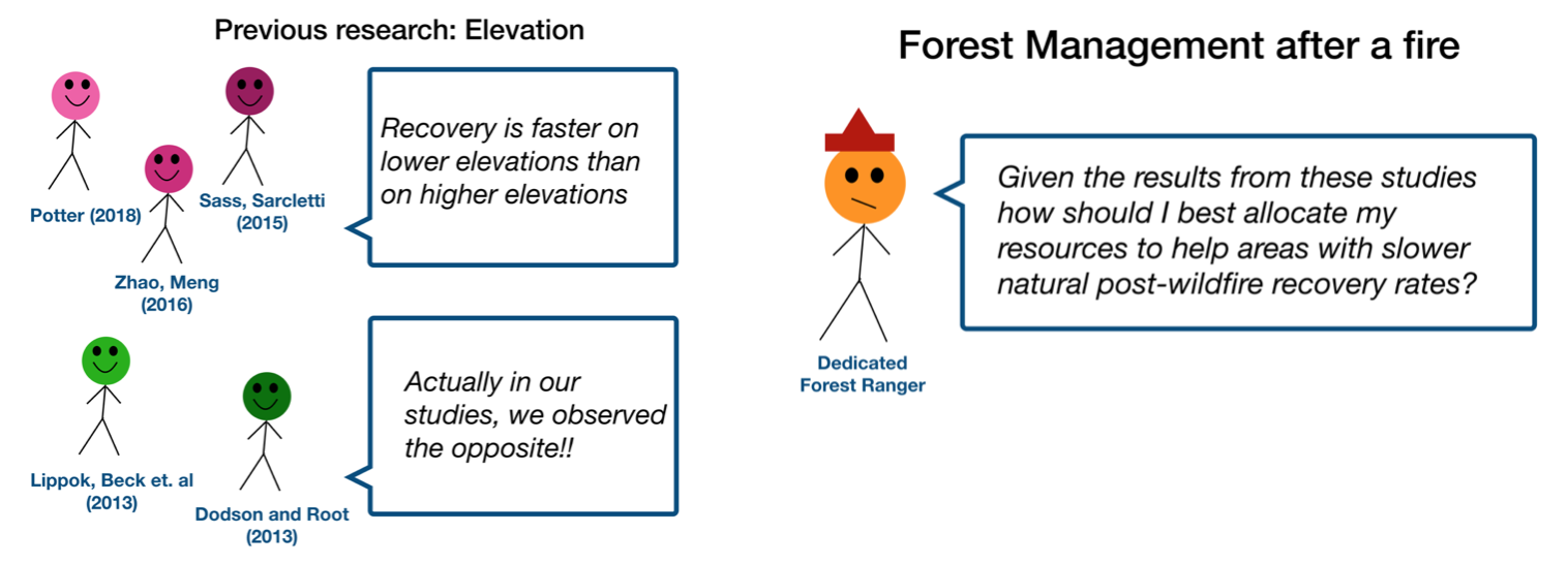
Orient the audience and draw them in by demonstrating the relevance and importance of your research story with strong global motive. Provide them with the necessary vocabulary and background knowledge to understand the plot of your story. Introduce the key studies (characters) relevant in your story and build tension and conflict with scholarly and data motive. By the end of your introduction, your audience should clearly understand your research question and be dying to know how you resolve the tension built through motive.

• Methods (rising action)

The methods section should transition smoothly and logically from the introduction. Beware of presenting your methods in a boring, arc-killing, ‘this is what I did.’ Focus on the details that set your story apart from the stories other people have already told. Keep the audience interested by clearly motivating your decisions based on your original research question or the tension built in your introduction.

• Results (climax)

Less is usually more here. Only present results which are clearly related to the focused research question you are presenting. Make sure you explain the results clearly so that your audience understands what your research found. This is the peak of tension in your narrative arc, so don’t undercut it by quickly clicking through to your discussion.

• Discussion (falling action)

By now your audience should be dying for a satisfying resolution. Here is where you contextualize your results and begin resolving the tension between past research. Be thorough. If you have too many conflicts left unresolved, or you don’t have enough time to present all of the resolutions, you probably need to further narrow the scope of your presentation.

• Conclusion (denouement)

Return back to your initial research question and motive, resolving any final conflicts and tying up loose ends. Leave the audience with a clear resolution of your focus research question, and use unresolved tension to set up potential sequels (i.e. further research).

Use your medium to enhance the narrative

Visual presentations should be dominated by clear, intentional graphics. Subtle animation in key moments (usually during the results or discussion) can add drama to the narrative arc and make conflict resolutions more satisfying. You are narrating a story written in images, videos, cartoons, and graphs. While your paper is mostly text, with graphics to highlight crucial points, your slides should be the opposite. Adapting to the new medium may require you to create or acquire far more graphics than you included in your paper, but it is necessary to create an engaging presentation.

The most important thing you can do for your presentation is to practice and revise. Bother your friends, your roommates, TAs–anybody who will sit down and listen to your work. Beyond that, think about presentations you have found compelling and try to incorporate some of those elements into your own. Remember you want your work to be comprehensible; you aren’t creating experts in 10 minutes. Above all, try to stay passionate about what you did and why. You put the time in, so show your audience that it’s worth it.

For more insight into research presentations, check out these past PCUR posts written by Emma and Ellie .

— Alec Getraer, Natural Sciences Correspondent

Share this:

• Share on Tumblr

Reference management. Clean and simple.

How to make a scientific presentation

Scientific presentation outlines

Questions to ask yourself before you write your talk, 1. how much time do you have, 2. who will you speak to, 3. what do you want the audience to learn from your talk, step 1: outline your presentation, step 2: plan your presentation slides, step 3: make the presentation slides, slide design, text elements, animations and transitions, step 4: practice your presentation, final thoughts, frequently asked questions about preparing scientific presentations, related articles.

A good scientific presentation achieves three things: you communicate the science clearly, your research leaves a lasting impression on your audience, and you enhance your reputation as a scientist.

But, what is the best way to prepare for a scientific presentation? How do you start writing a talk? What details do you include, and what do you leave out?

It’s tempting to launch into making lots of slides. But, starting with the slides can mean you neglect the narrative of your presentation, resulting in an overly detailed, boring talk.

The key to making an engaging scientific presentation is to prepare the narrative of your talk before beginning to construct your presentation slides. Planning your talk will ensure that you tell a clear, compelling scientific story that will engage the audience.

In this guide, you’ll find everything you need to know to make a good oral scientific presentation, including:

• The different types of oral scientific presentations and how they are delivered;
• How to outline a scientific presentation;
• How to make slides for a scientific presentation.

Our advice results from delving into the literature on writing scientific talks and from our own experiences as scientists in giving and listening to presentations. We provide tips and best practices for giving scientific talks in a separate post.

There are two main types of scientific talks:

• Your talk focuses on a single study . Typically, you tell the story of a single scientific paper. This format is common for short talks at contributed sessions in conferences.
• Your talk describes multiple studies. You tell the story of multiple scientific papers. It is crucial to have a theme that unites the studies, for example, an overarching question or problem statement, with each study representing specific but different variations of the same theme. Typically, PhD defenses, invited seminars, lectures, or talks for a prospective employer (i.e., “job talks”) fall into this category.

➡️ Learn how to prepare an excellent thesis defense

The length of time you are allotted for your talk will determine whether you will discuss a single study or multiple studies, and which details to include in your story.

The background and interests of your audience will determine the narrative direction of your talk, and what devices you will use to get their attention. Will you be speaking to people specializing in your field, or will the audience also contain people from disciplines other than your own? To reach non-specialists, you will need to discuss the broader implications of your study outside your field.

The needs of the audience will also determine what technical details you will include, and the language you will use. For example, an undergraduate audience will have different needs than an audience of seasoned academics. Students will require a more comprehensive overview of background information and explanations of jargon but will need less technical methodological details.

Your goal is to speak to the majority. But, make your talk accessible to the least knowledgeable person in the room.

This is called the thesis statement, or simply the “take-home message”. Having listened to your talk, what message do you want the audience to take away from your presentation? Describe the main idea in one or two sentences. You want this theme to be present throughout your presentation. Again, the thesis statement will depend on the audience and the type of talk you are giving.

Your thesis statement will drive the narrative for your talk. By deciding the take-home message you want to convince the audience of as a result of listening to your talk, you decide how the story of your talk will flow and how you will navigate its twists and turns. The thesis statement tells you the results you need to show, which subsequently tells you the methods or studies you need to describe, which decides the angle you take in your introduction.

➡️ Learn how to write a thesis statement

The goal of your talk is that the audience leaves afterward with a clear understanding of the key take-away message of your research. To achieve that goal, you need to tell a coherent, logical story that conveys your thesis statement throughout the presentation. You can tell your story through careful preparation of your talk.

Preparation of a scientific presentation involves three separate stages: outlining the scientific narrative, preparing slides, and practicing your delivery. Making the slides of your talk without first planning what you are going to say is inefficient.

Here, we provide a 4 step guide to writing your scientific presentation:

• Outline your presentation
• Plan your presentation slides
• Make the presentation slides
• Practice your presentation

Writing an outline helps you consider the key pieces of your talk and how they fit together from the beginning, preventing you from forgetting any important details. It also means you avoid changing the order of your slides multiple times, saving you time.

Plan your talk as discrete sections. In the table below, we describe the sections for a single study talk vs. a talk discussing multiple studies:

The following tips apply when writing the outline of a single study talk. You can easily adapt this framework if you are writing a talk discussing multiple studies.

Introduction: Writing the introduction can be the hardest part of writing a talk. And when giving it, it’s the point where you might be at your most nervous. But preparing a good, concise introduction will settle your nerves.

The introduction tells the audience the story of why you studied your topic. A good introduction succinctly achieves four things, in the following order.

• It gives a broad perspective on the problem or topic for people in the audience who may be outside your discipline (i.e., it explains the big-picture problem motivating your study).
• It describes why you did the study, and why the audience should care.
• It gives a brief indication of how your study addressed the problem and provides the necessary background information that the audience needs to understand your work.
• It indicates what the audience will learn from the talk, and prepares them for what will come next.

A good introduction not only gives the big picture and motivations behind your study but also concisely sets the stage for what the audience will learn from the talk (e.g., the questions your work answers, and/or the hypotheses that your work tests). The end of the introduction will lead to a natural transition to the methods.

Give a broad perspective on the problem. The easiest way to start with the big picture is to think of a hook for the first slide of your presentation. A hook is an opening that gets the audience’s attention and gets them interested in your story. In science, this might take the form of a why, or a how question, or it could be a statement about a major problem or open question in your field. Other examples of hooks include quotes, short anecdotes, or interesting statistics.

Why should the audience care? Next, decide on the angle you are going to take on your hook that links to the thesis of your talk. In other words, you need to set the context, i.e., explain why the audience should care. For example, you may introduce an observation from nature, a pattern in experimental data, or a theory that you want to test. The audience must understand your motivations for the study.

Supplementary details. Once you have established the hook and angle, you need to include supplementary details to support them. For example, you might state your hypothesis. Then go into previous work and the current state of knowledge. Include citations of these studies. If you need to introduce some technical methodological details, theory, or jargon, do it here.

Conclude your introduction. The motivation for the work and background information should set the stage for the conclusion of the introduction, where you describe the goals of your study, and any hypotheses or predictions. Let the audience know what they are going to learn.

Methods: The audience will use your description of the methods to assess the approach you took in your study and to decide whether your findings are credible. Tell the story of your methods in chronological order. Use visuals to describe your methods as much as possible. If you have equations, make sure to take the time to explain them. Decide what methods to include and how you will show them. You need enough detail so that your audience will understand what you did and therefore can evaluate your approach, but avoid including superfluous details that do not support your main idea. You want to avoid the common mistake of including too much data, as the audience can read the paper(s) later.

Results: This is the evidence you present for your thesis. The audience will use the results to evaluate the support for your main idea. Choose the most important and interesting results—those that support your thesis. You don’t need to present all the results from your study (indeed, you most likely won’t have time to present them all). Break down complex results into digestible pieces, e.g., comparisons over multiple slides (more tips in the next section).

Summary: Summarize your main findings. Displaying your main findings through visuals can be effective. Emphasize the new contributions to scientific knowledge that your work makes.

Conclusion: Complete the circle by relating your conclusions to the big picture topic in your introduction—and your hook, if possible. It’s important to describe any alternative explanations for your findings. You might also speculate on future directions arising from your research. The slides that comprise your conclusion do not need to state “conclusion”. Rather, the concluding slide title should be a declarative sentence linking back to the big picture problem and your main idea.

It’s important to end well by planning a strong closure to your talk, after which you will thank the audience. Your closing statement should relate to your thesis, perhaps by stating it differently or memorably. Avoid ending awkwardly by memorizing your closing sentence.

By now, you have an outline of the story of your talk, which you can use to plan your slides. Your slides should complement and enhance what you will say. Use the following steps to prepare your slides.

• Write the slide titles to match your talk outline. These should be clear and informative declarative sentences that succinctly give the main idea of the slide (e.g., don’t use “Methods” as a slide title). Have one major idea per slide. In a YouTube talk on designing effective slides , researcher Michael Alley shows examples of instructive slide titles.
• Decide how you will convey the main idea of the slide (e.g., what figures, photographs, equations, statistics, references, or other elements you will need). The body of the slide should support the slide’s main idea.
• Under each slide title, outline what you want to say, in bullet points.

In sum, for each slide, prepare a title that summarizes its major idea, a list of visual elements, and a summary of the points you will make. Ensure each slide connects to your thesis. If it doesn’t, then you don’t need the slide.

Slides for scientific presentations have three major components: text (including labels and legends), graphics, and equations. Here, we give tips on how to present each of these components.

• Have an informative title slide. Include the names of all coauthors and their affiliations. Include an attractive image relating to your study.
• Make the foreground content of your slides “pop” by using an appropriate background. Slides that have white backgrounds with black text work well for small rooms, whereas slides with black backgrounds and white text are suitable for large rooms.
• The layout of your slides should be simple. Pay attention to how and where you lay the visual and text elements on each slide. It’s tempting to cram information, but you need lots of empty space. Retain space at the sides and bottom of your slides.
• Use sans serif fonts with a font size of at least 20 for text, and up to 40 for slide titles. Citations can be in 14 font and should be included at the bottom of the slide.
• Use bold or italics to emphasize words, not underlines or caps. Keep these effects to a minimum.
• Use concise text . You don’t need full sentences. Convey the essence of your message in as few words as possible. Write down what you’d like to say, and then shorten it for the slide. Remove unnecessary filler words.
• Text blocks should be limited to two lines. This will prevent you from crowding too much information on the slide.
• Include names of technical terms in your talk slides, especially if they are not familiar to everyone in the audience.
• Proofread your slides. Typos and grammatical errors are distracting for your audience.
• Include citations for the hypotheses or observations of other scientists.
• Good figures and graphics are essential to sustain audience interest. Use graphics and photographs to show the experiment or study system in action and to explain abstract concepts.
• Don’t use figures straight from your paper as they may be too detailed for your talk, and details like axes may be too small. Make new versions if necessary. Make them large enough to be visible from the back of the room.
• Use graphs to show your results, not tables. Tables are difficult for your audience to digest! If you must present a table, keep it simple.
• Label the axes of graphs and indicate the units. Label important components of graphics and photographs and include captions. Include sources for graphics that are not your own.
• Explain all the elements of a graph. This includes the axes, what the colors and markers mean, and patterns in the data.
• Use colors in figures and text in a meaningful, not random, way. For example, contrasting colors can be effective for pointing out comparisons and/or differences. Don’t use neon colors or pastels.
• Use thick lines in figures, and use color to create contrasts in the figures you present. Don’t use red/green or red/blue combinations, as color-blind audience members can’t distinguish between them.
• Arrows or circles can be effective for drawing attention to key details in graphs and equations. Add some text annotations along with them.
• Write your summary and conclusion slides using graphics, rather than showing a slide with a list of bullet points. Showing some of your results again can be helpful to remind the audience of your message.
• If your talk has equations, take time to explain them. Include text boxes to explain variables and mathematical terms, and put them under each term in the equation.
• Combine equations with a graphic that shows the scientific principle, or include a diagram of the mathematical model.
• Use animations judiciously. They are helpful to reveal complex ideas gradually, for example, if you need to make a comparison or contrast or to build a complicated argument or figure. For lists, reveal one bullet point at a time. New ideas appearing sequentially will help your audience follow your logic.
• Slide transitions should be simple. Silly ones distract from your message.
• Decide how you will make the transition as you move from one section of your talk to the next. For example, if you spend time talking through details, provide a summary afterward, especially in a long talk. Another common tactic is to have a “home slide” that you return to multiple times during the talk that reinforces your main idea or message. In her YouTube talk on designing effective scientific presentations , Stanford biologist Susan McConnell suggests using the approach of home slides to build a cohesive narrative.

To deliver a polished presentation, it is essential to practice it. Here are some tips.

• For your first run-through, practice alone. Pay attention to your narrative. Does your story flow naturally? Do you know how you will start and end? Are there any awkward transitions? Do animations help you tell your story? Do your slides help to convey what you are saying or are they missing components?
• Next, practice in front of your advisor, and/or your peers (e.g., your lab group). Ask someone to time your talk. Take note of their feedback and the questions that they ask you (you might be asked similar questions during your real talk).
• Edit your talk, taking into account the feedback you’ve received. Eliminate superfluous slides that don’t contribute to your takeaway message.
• Practice as many times as needed to memorize the order of your slides and the key transition points of your talk. However, don’t try to learn your talk word for word. Instead, memorize opening and closing statements, and sentences at key junctures in the presentation. Your presentation should resemble a serious but spontaneous conversation with the audience.
• Practicing multiple times also helps you hone the delivery of your talk. While rehearsing, pay attention to your vocal intonations and speed. Make sure to take pauses while you speak, and make eye contact with your imaginary audience.
• Make sure your talk finishes within the allotted time, and remember to leave time for questions. Conferences are particularly strict on run time.
• Anticipate questions and challenges from the audience, and clarify ambiguities within your slides and/or speech in response.
• If you anticipate that you could be asked questions about details but you don’t have time to include them, or they detract from the main message of your talk, you can prepare slides that address these questions and place them after the final slide of your talk.

➡️ More tips for giving scientific presentations

An organized presentation with a clear narrative will help you communicate your ideas effectively, which is essential for engaging your audience and conveying the importance of your work. Taking time to plan and outline your scientific presentation before writing the slides will help you manage your nerves and feel more confident during the presentation, which will improve your overall performance.

A good scientific presentation has an engaging scientific narrative with a memorable take-home message. It has clear, informative slides that enhance what the speaker says. You need to practice your talk many times to ensure you deliver a polished presentation.

First, consider who will attend your presentation, and what you want the audience to learn about your research. Tailor your content to their level of knowledge and interests. Second, create an outline for your presentation, including the key points you want to make and the evidence you will use to support those points. Finally, practice your presentation several times to ensure that it flows smoothly and that you are comfortable with the material.

Prepare an opening that immediately gets the audience’s attention. A common device is a why or a how question, or a statement of a major open problem in your field, but you could also start with a quote, interesting statistic, or case study from your field.

Scientific presentations typically either focus on a single study (e.g., a 15-minute conference presentation) or tell the story of multiple studies (e.g., a PhD defense or 50-minute conference keynote talk). For a single study talk, the structure follows the scientific paper format: Introduction, Methods, Results, Summary, and Conclusion, whereas the format of a talk discussing multiple studies is more complex, but a theme unifies the studies.

Ensure you have one major idea per slide, and convey that idea clearly (through images, equations, statistics, citations, video, etc.). The slide should include a title that summarizes the major point of the slide, should not contain too much text or too many graphics, and color should be used meaningfully.

• Publication Recognition

How to Make a PowerPoint Presentation of Your Research Paper

• 4 minute read
• 121.4K views

Table of Contents

A research paper presentation is often used at conferences and in other settings where you have an opportunity to share your research, and get feedback from your colleagues. Although it may seem as simple as summarizing your research and sharing your knowledge, successful research paper PowerPoint presentation examples show us that there’s a little bit more than that involved.

In this article, we’ll highlight how to make a PowerPoint presentation from a research paper, and what to include (as well as what NOT to include). We’ll also touch on how to present a research paper at a conference.

Purpose of a Research Paper Presentation

The purpose of presenting your paper at a conference or forum is different from the purpose of conducting your research and writing up your paper. In this setting, you want to highlight your work instead of including every detail of your research. Likewise, a presentation is an excellent opportunity to get direct feedback from your colleagues in the field. But, perhaps the main reason for presenting your research is to spark interest in your work, and entice the audience to read your research paper.

So, yes, your presentation should summarize your work, but it needs to do so in a way that encourages your audience to seek out your work, and share their interest in your work with others. It’s not enough just to present your research dryly, to get information out there. More important is to encourage engagement with you, your research, and your work.

Tips for Creating Your Research Paper Presentation

In addition to basic PowerPoint presentation recommendations, which we’ll cover later in this article, think about the following when you’re putting together your research paper presentation:

• Know your audience : First and foremost, who are you presenting to? Students? Experts in your field? Potential funders? Non-experts? The truth is that your audience will probably have a bit of a mix of all of the above. So, make sure you keep that in mind as you prepare your presentation.

Know more about: Discover the Target Audience .

• Your audience is human : In other words, they may be tired, they might be wondering why they’re there, and they will, at some point, be tuning out. So, take steps to help them stay interested in your presentation. You can do that by utilizing effective visuals, summarize your conclusions early, and keep your research easy to understand.
• Running outline : It’s not IF your audience will drift off, or get lost…it’s WHEN. Keep a running outline, either within the presentation or via a handout. Use visual and verbal clues to highlight where you are in the presentation.
• Where does your research fit in? You should know of work related to your research, but you don’t have to cite every example. In addition, keep references in your presentation to the end, or in the handout. Your audience is there to hear about your work.
• Plan B : Anticipate possible questions for your presentation, and prepare slides that answer those specific questions in more detail, but have them at the END of your presentation. You can then jump to them, IF needed.

What Makes a PowerPoint Presentation Effective?

You’ve probably attended a presentation where the presenter reads off of their PowerPoint outline, word for word. Or where the presentation is busy, disorganized, or includes too much information. Here are some simple tips for creating an effective PowerPoint Presentation.

• Less is more: You want to give enough information to make your audience want to read your paper. So include details, but not too many, and avoid too many formulas and technical jargon.
• Clean and professional : Avoid excessive colors, distracting backgrounds, font changes, animations, and too many words. Instead of whole paragraphs, bullet points with just a few words to summarize and highlight are best.
• Know your real-estate : Each slide has a limited amount of space. Use it wisely. Typically one, no more than two points per slide. Balance each slide visually. Utilize illustrations when needed; not extraneously.
• Keep things visual : Remember, a PowerPoint presentation is a powerful tool to present things visually. Use visual graphs over tables and scientific illustrations over long text. Keep your visuals clean and professional, just like any text you include in your presentation.

Know more about our Scientific Illustrations Services .

Another key to an effective presentation is to practice, practice, and then practice some more. When you’re done with your PowerPoint, go through it with friends and colleagues to see if you need to add (or delete excessive) information. Double and triple check for typos and errors. Know the presentation inside and out, so when you’re in front of your audience, you’ll feel confident and comfortable.

How to Present a Research Paper

If your PowerPoint presentation is solid, and you’ve practiced your presentation, that’s half the battle. Follow the basic advice to keep your audience engaged and interested by making eye contact, encouraging questions, and presenting your information with enthusiasm.

We encourage you to read our articles on how to present a scientific journal article and tips on giving good scientific presentations .

Language Editing Plus

Improve the flow and writing of your research paper with Language Editing Plus. This service includes unlimited editing, manuscript formatting for the journal of your choice, reference check and even a customized cover letter. Learn more here , and get started today!

• Manuscript Preparation

Know How to Structure Your PhD Thesis

• Research Process

Systematic Literature Review or Literature Review?

You may also like.

What is a Good H-index?

What is a Corresponding Author?

How to Submit a Paper for Publication in a Journal

Input your search keywords and press Enter.

Home Blog Presentation Ideas How to Create and Deliver a Research Presentation

How to Create and Deliver a Research Presentation

Every research endeavor ends up with the communication of its findings. Graduate-level research culminates in a thesis defense , while many academic and scientific disciplines are published in peer-reviewed journals. In a business context, PowerPoint research presentation is the default format for reporting the findings to stakeholders.

Condensing months of work into a few slides can prove to be challenging. It requires particular skills to create and deliver a research presentation that promotes informed decisions and drives long-term projects forward.

Table of Contents

What is a Research Presentation

Key slides for creating a research presentation, tips when delivering a research presentation, how to present sources in a research presentation, recommended templates to create a research presentation.

A research presentation is the communication of research findings, typically delivered to an audience of peers, colleagues, students, or professionals. In the academe, it is meant to showcase the importance of the research paper , state the findings and the analysis of those findings, and seek feedback that could further the research.

The presentation of research becomes even more critical in the business world as the insights derived from it are the basis of strategic decisions of organizations. Information from this type of report can aid companies in maximizing the sales and profit of their business. Major projects such as research and development (R&D) in a new field, the launch of a new product or service, or even corporate social responsibility (CSR) initiatives will require the presentation of research findings to prove their feasibility.

Market research and technical research are examples of business-type research presentations you will commonly encounter.

In this article, we’ve compiled all the essential tips, including some examples and templates, to get you started with creating and delivering a stellar research presentation tailored specifically for the business context.

Various research suggests that the average attention span of adults during presentations is around 20 minutes, with a notable drop in an engagement at the 10-minute mark . Beyond that, you might see your audience doing other things.

How can you avoid such a mistake? The answer lies in the adage “keep it simple, stupid” or KISS. We don’t mean dumbing down your content but rather presenting it in a way that is easily digestible and accessible to your audience. One way you can do this is by organizing your research presentation using a clear structure.

Here are the slides you should prioritize when creating your research presentation PowerPoint.

1.  Title Page

The title page is the first thing your audience will see during your presentation, so put extra effort into it to make an impression. Of course, writing presentation titles and title pages will vary depending on the type of presentation you are to deliver. In the case of a research presentation, you want a formal and academic-sounding one. It should include:

• The full title of the report
• The date of the report
• The name of the researchers or department in charge of the report
• The name of the organization for which the presentation is intended

When writing the title of your research presentation, it should reflect the topic and objective of the report. Focus only on the subject and avoid adding redundant phrases like “A research on” or “A study on.” However, you may use phrases like “Market Analysis” or “Feasibility Study” because they help identify the purpose of the presentation. Doing so also serves a long-term purpose for the filing and later retrieving of the document.

Here’s a sample title page for a hypothetical market research presentation from Gillette .

2. Executive Summary Slide

The executive summary marks the beginning of the body of the presentation, briefly summarizing the key discussion points of the research. Specifically, the summary may state the following:

• The purpose of the investigation and its significance within the organization’s goals
• The methods used for the investigation
• The major findings of the investigation
• The conclusions and recommendations after the investigation

Although the executive summary encompasses the entry of the research presentation, it should not dive into all the details of the work on which the findings, conclusions, and recommendations were based. Creating the executive summary requires a focus on clarity and brevity, especially when translating it to a PowerPoint document where space is limited.

Each point should be presented in a clear and visually engaging manner to capture the audience’s attention and set the stage for the rest of the presentation. Use visuals, bullet points, and minimal text to convey information efficiently.

3. Introduction/ Project Description Slides

In this section, your goal is to provide your audience with the information that will help them understand the details of the presentation. Provide a detailed description of the project, including its goals, objectives, scope, and methods for gathering and analyzing data.

You want to answer these fundamental questions:

• What specific questions are you trying to answer, problems you aim to solve, or opportunities you seek to explore?
• Why is this project important, and what prompted it?
• What are the boundaries of your research or initiative? 
• How were the data gathered?

Important: The introduction should exclude specific findings, conclusions, and recommendations.

4. Data Presentation and Analyses Slides

This is the longest section of a research presentation, as you’ll present the data you’ve gathered and provide a thorough analysis of that data to draw meaningful conclusions. The format and components of this section can vary widely, tailored to the specific nature of your research.

For example, if you are doing market research, you may include the market potential estimate, competitor analysis, and pricing analysis. These elements will help your organization determine the actual viability of a market opportunity.

Visual aids like charts, graphs, tables, and diagrams are potent tools to convey your key findings effectively. These materials may be numbered and sequenced (Figure 1, Figure 2, and so forth), accompanied by text to make sense of the insights.

5. Conclusions

The conclusion of a research presentation is where you pull together the ideas derived from your data presentation and analyses in light of the purpose of the research. For example, if the objective is to assess the market of a new product, the conclusion should determine the requirements of the market in question and tell whether there is a product-market fit.

Designing your conclusion slide should be straightforward and focused on conveying the key takeaways from your research. Keep the text concise and to the point. Present it in bullet points or numbered lists to make the content easily scannable.

6. Recommendations

The findings of your research might reveal elements that may not align with your initial vision or expectations. These deviations are addressed in the recommendations section of your presentation, which outlines the best course of action based on the result of the research.

What emerging markets should we target next? Do we need to rethink our pricing strategies? Which professionals should we hire for this special project? — these are some of the questions that may arise when coming up with this part of the research.

Recommendations may be combined with the conclusion, but presenting them separately to reinforce their urgency. In the end, the decision-makers in the organization or your clients will make the final call on whether to accept or decline the recommendations.

7. Questions Slide

Members of your audience are not involved in carrying out your research activity, which means there’s a lot they don’t know about its details. By offering an opportunity for questions, you can invite them to bridge that gap, seek clarification, and engage in a dialogue that enhances their understanding.

If your research is more business-oriented, facilitating a question and answer after your presentation becomes imperative as it’s your final appeal to encourage buy-in for your recommendations.

A simple “Ask us anything” slide can indicate that you are ready to accept questions.

1. Focus on the Most Important Findings

The truth about presenting research findings is that your audience doesn’t need to know everything. Instead, they should receive a distilled, clear, and meaningful overview that focuses on the most critical aspects.

You will likely have to squeeze in the oral presentation of your research into a 10 to 20-minute presentation, so you have to make the most out of the time given to you. In the presentation, don’t soak in the less important elements like historical backgrounds. Decision-makers might even ask you to skip these portions and focus on sharing the findings.

2. Do Not Read Word-per-word

Reading word-for-word from your presentation slides intensifies the danger of losing your audience’s interest. Its effect can be detrimental, especially if the purpose of your research presentation is to gain approval from the audience. So, how can you avoid this mistake?

• Make a conscious design decision to keep the text on your slides minimal. Your slides should serve as visual cues to guide your presentation.
• Structure your presentation as a narrative or story. Stories are more engaging and memorable than dry, factual information.
• Prepare speaker notes with the key points of your research. Glance at it when needed.
• Engage with the audience by maintaining eye contact and asking rhetorical questions.

3. Don’t Go Without Handouts

Handouts are paper copies of your presentation slides that you distribute to your audience. They typically contain the summary of your key points, but they may also provide supplementary information supporting data presented through tables and graphs.

The purpose of distributing presentation handouts is to easily retain the key points you presented as they become good references in the future. Distributing handouts in advance allows your audience to review the material and come prepared with questions or points for discussion during the presentation.

4. Actively Listen

An equally important skill that a presenter must possess aside from speaking is the ability to listen. We are not just talking about listening to what the audience is saying but also considering their reactions and nonverbal cues. If you sense disinterest or confusion, you can adapt your approach on the fly to re-engage them.

For example, if some members of your audience are exchanging glances, they may be skeptical of the research findings you are presenting. This is the best time to reassure them of the validity of your data and provide a concise overview of how it came to be. You may also encourage them to seek clarification.

5. Be Confident

Anxiety can strike before a presentation – it’s a common reaction whenever someone has to speak in front of others. If you can’t eliminate your stress, try to manage it.

People hate public speaking not because they simply hate it. Most of the time, it arises from one’s belief in themselves. You don’t have to take our word for it. Take Maslow’s theory that says a threat to one’s self-esteem is a source of distress among an individual.

Now, how can you master this feeling? You’ve spent a lot of time on your research, so there is no question about your topic knowledge. Perhaps you just need to rehearse your research presentation. If you know what you will say and how to say it, you will gain confidence in presenting your work.

All sources you use in creating your research presentation should be given proper credit. The APA Style is the most widely used citation style in formal research.

In-text citation

Add references within the text of your presentation slide by giving the author’s last name, year of publication, and page number (if applicable) in parentheses after direct quotations or paraphrased materials. As in:

The alarming rate at which global temperatures rise directly impacts biodiversity (Smith, 2020, p. 27).

If the author’s name and year of publication are mentioned in the text, add only the page number in parentheses after the quotations or paraphrased materials. As in:

According to Smith (2020), the alarming rate at which global temperatures rise directly impacts biodiversity (p. 27).

Image citation

All images from the web, including photos, graphs, and tables, used in your slides should be credited using the format below.

Creator’s Last Name, First Name. “Title of Image.” Website Name, Day Mo. Year, URL. Accessed Day Mo. Year.

Work cited page

A work cited page or reference list should follow after the last slide of your presentation. The list should be alphabetized by the author’s last name and initials followed by the year of publication, the title of the book or article, the place of publication, and the publisher. As in:

Smith, J. A. (2020). Climate Change and Biodiversity: A Comprehensive Study. New York, NY: ABC Publications.

When citing a document from a website, add the source URL after the title of the book or article instead of the place of publication and the publisher. As in:

Smith, J. A. (2020). Climate Change and Biodiversity: A Comprehensive Study. Retrieved from https://www.smith.com/climate-change-and-biodiversity.

1. Research Project Presentation PowerPoint Template

A slide deck containing 18 different slides intended to take off the weight of how to make a research presentation. With tons of visual aids, presenters can reference existing research on similar projects to this one – or link another research presentation example – provide an accurate data analysis, disclose the methodology used, and much more.

Use This Template

2. Research Presentation Scientific Method Diagram PowerPoint Template

Whenever you intend to raise questions, expose the methodology you used for your research, or even suggest a scientific method approach for future analysis, this circular wheel diagram is a perfect fit for any presentation study.

Customize all of its elements to suit the demands of your presentation in just minutes.

3. Thesis Research Presentation PowerPoint Template

If your research presentation project belongs to academia, then this is the slide deck to pair that presentation. With a formal aesthetic and minimalistic style, this research presentation template focuses only on exposing your information as clearly as possible.

Use its included bar charts and graphs to introduce data, change the background of each slide to suit the topic of your presentation, and customize each of its elements to meet the requirements of your project with ease.

4. Animated Research Cards PowerPoint Template

Visualize ideas and their connection points with the help of this research card template for PowerPoint. This slide deck, for example, can help speakers talk about alternative concepts to what they are currently managing and its possible outcomes, among different other usages this versatile PPT template has. Zoom Animation effects make a smooth transition between cards (or ideas).

5. Research Presentation Slide Deck for PowerPoint

With a distinctive professional style, this research presentation PPT template helps business professionals and academics alike to introduce the findings of their work to team members or investors.

By accessing this template, you get the following slides:

• Introduction
• Problem Statement
• Research Questions
• Conceptual Research Framework (Concepts, Theories, Actors, & Constructs)
• Study design and methods
• Population & Sampling
• Data Collection
• Data Analysis

Check it out today and craft a powerful research presentation out of it!

A successful research presentation in business is not just about presenting data; it’s about persuasion to take meaningful action. It’s the bridge that connects your research efforts to the strategic initiatives of your organization. To embark on this journey successfully, planning your presentation thoroughly is paramount, from designing your PowerPoint to the delivery.

Take a look and get inspiration from the sample research presentation slides above, put our tips to heart, and transform your research findings into a compelling call to action.

Like this article? Please share

Academics, Presentation Approaches, Research & Development Filed under Presentation Ideas

Related Articles

Filed under Design • March 27th, 2024

How to Make a Presentation Graph

Detailed step-by-step instructions to master the art of how to make a presentation graph in PowerPoint and Google Slides. Check it out!

Filed under Presentation Ideas • February 29th, 2024

How to Make a Fundraising Presentation (with Thermometer Templates & Slides)

Meet a new framework to design fundraising presentations by harnessing the power of fundraising thermometer templates. Detailed guide with examples.

Filed under Presentation Ideas • February 15th, 2024

How to Create a 5 Minutes Presentation

Master the art of short-format speeches like the 5 minutes presentation with this article. Insights on content structure, audience engagement and more.

Leave a Reply

• Locations and Hours
• UCLA Library
• Research Guides
• Research Tips and Tools

Advanced Research Methods

• Presenting the Research Paper
• What Is Research?
• Library Research
• Writing a Research Proposal
• Writing the Research Paper

Writing an Abstract

Oral presentation, compiling a powerpoint.

Abstract : a short statement that describes a longer work.

• Indicate the subject.
• Describe the purpose of the investigation.
• Briefly discuss the method used.
• Make a statement about the result.

Oral presentations usually introduce a discussion of a topic or research paper. A good oral presentation is focused, concise, and interesting in order to trigger a discussion.

• Be well prepared; write a detailed outline.
• Introduce the subject.
• Talk about the sources and the method.
• Indicate if there are conflicting views about the subject (conflicting views trigger discussion).
• Make a statement about your new results (if this is your research paper).
• Use visual aids or handouts if appropriate.

An effective PowerPoint presentation is just an aid to the presentation, not the presentation itself .

• Be brief and concise.
• Focus on the subject.
• Attract attention; indicate interesting details.
• If possible, use relevant visual illustrations (pictures, maps, charts graphs, etc.).
• Use bullet points or numbers to structure the text.
• Make clear statements about the essence/results of the topic/research.
• Don't write down the whole outline of your paper and nothing else.
• Don't write long full sentences on the slides.
• Don't use distracting colors, patterns, pictures, decorations on the slides.
• Don't use too complicated charts, graphs; only those that are relatively easy to understand.
• << Previous: Writing the Research Paper
• Last Updated: Jan 4, 2024 12:24 PM
• URL: https://guides.library.ucla.edu/research-methods

• Event Website Publish a modern and mobile friendly event website.
• Registration & Payments Collect registrations & online payments for your event.
• Abstract Management Collect and manage all your abstract submissions.
• Peer Reviews Easily distribute and manage your peer reviews.
• Conference Program Effortlessly build & publish your event program.
• Virtual Poster Sessions Host engaging virtual poster sessions.
• Customer Success Stories
• Wall of Love ❤️

How to Present Your Research (Guidelines and Tips)

Published on 01 Feb 2023

Presenting at a conference can be stressful, but can lead to many opportunities, which is why coming prepared is super beneficial.

The internet is full to the brim with tips for making a good presentation. From what you wear to how you stand to good slide design, there’s no shortage of advice to make any old presentation come to life. 

But, not all presentations are created equal. Research presentations, in particular, are unique. 

Communicating complex concepts to an audience with a varied range of awareness about your research topic can be tricky. A lack of guidance and preparation can ruin your chance to share important information with a conference community. This could mean lost opportunities in collaboration or funding or lost confidence in yourself and your work.

So, we’ve put together a list of tips with research presentations in mind. Here’s our top to-do’s when preparing to present your research.

Take every research presentation opportunity

The worst thing you could do for your research is to not present it at all. As intimidating as it can be to get up in front of an audience, you shouldn’t let that stop you from seizing a good opportunity to share your work with a wider community.

These contestants from the Vitae Three Minute Thesis Competition have some great advice to share on taking every possible chance to talk about your research. 

Double-check your research presentation guidelines

Before you get started on your presentation, double-check if you’ve been given guidelines for it. 

If you don’t have specific guidelines for the context of your presentation, we’ve put together a general outline to help you get started. It’s made with the assumption of a 10-15 minute presentation time. So, if you have longer to present, you can always extend important sections or talk longer on certain slides:

• Title Slide (1 slide) - This is a placeholder to give some visual interest and display the topic until your presentation begins.
• Short Introduction (2-3 slides) - This is where you pique the interest of your audience and establish the key questions your presentation covers. Give context to your study with a brief review of the literature (focus on key points, not a full review). If your study relates to any particularly relevant issues, mention it here to increase the audience's interest in the topic.
• Hypothesis (1 slide) - Clearly state your hypothesis.
• Description of Methods (2-3 slides) - Clearly, but briefly, summarize your study design including a clear description of the study population, the sample size and any instruments or manipulations to gather the data.
• Results and Data Interpretation (2-4 slides) - Illustrate your results through simple tables, graphs, and images. Remind the audience of your hypothesis and discuss your interpretation of the data/results.
• Conclusion (2-3 slides) - Further interpret your results. If you had any sources of error or difficulties with your methods, discuss them here and address how they could be (or were) improved. Discuss your findings as part of the bigger picture and connect them to potential further outcomes or areas of study.
• Closing (1 slide) - If anyone supported your research with guidance, awards, or funding, be sure to recognize their contribution. If your presentation includes a Q&A session, open the floor to questions.

Plan for about one minute for each slide of information that you have. Be sure that you don’t cram your slides with text (stick to bullet points and images to emphasize key points).

And, if you’re looking for more inspiration to help you in scripting an oral research presentation. University of Virginia has a helpful oral presentation outline script .

A PhD Student working on an upcoming oral presentation.

Put yourself in your listeners shoes

As mentioned in the intro, research presentations are unique because they deal with specialized topics and complicated concepts. There’s a good chance that a large section of your audience won’t have the same understanding of your topic area as you do. So, do your best to understand where your listeners are at and adapt your language/definitions to that.

There’s an increasing awareness around the importance of scientific communication. Comms experts have even started giving TED Talks on how to bridge the gap between science and the public (check out Talk Nerdy to Me ). A general communication tip is to find out what sort of audience will listen to your talk. Then, beware of using jargon and acronyms unless you're 100% certain that your audience knows what they mean. 

On the other end of the spectrum, you don’t want to underestimate your audience. Giving too much background or spending ages summarizing old work to a group of experts in the field would be a waste of valuable presentation time (and would put you at risk of losing your audience's interest). 

Finally, if you can, practice your presentation on someone with a similar level of topic knowledge to the audience you’ll be presenting to.

Use scientific storytelling in your presentation

In scenarios where it’s appropriate, crafting a story allows you to break free from the often rigid tone of scientific communications. It helps your brain hit the refresh button and observe your findings from a new perspective. Plus, it can be a lot of fun to do!

If you have a chance to use scientific storytelling in your presentation, take full advantage of it. The best way to weave a story for your audience into a presentation is by setting the scene during your introduction. As you set the context of your research, set the context of your story/example at the same time. Continue drawing those parallels as you present. Then, deliver the main message of the story (or the “Aha!”) moment during your presentation’s conclusion.

If delivered well, a good story will keep your audience on the edge of their seats and glued to your entire presentation.

Emphasize the “Why” (not the “How”) of your research

Along the same lines as using storytelling, it’s important to think of WHY your audience should care about your work. Find ways to connect your research to valuable outcomes in society. Take your individual points on each slide and bring things back to the bigger picture. Constantly remind your listeners how it’s all connected and why that’s important.

One helpful way to get in this mindset is to look back to the moment before you became an expert on your topic. What got you interested? What was the reason for asking your research question? And, what motivated you to power through all the hard work to come? Then, looking forward, think about what key takeaways were most interesting or surprised you the most. How can these be applied to impact positive change in your research field or the wider community?

Be picky about what you include

It’s tempting to discuss all the small details of your methods or findings. Instead, focus on the most important information and takeaways that you think your audience will connect with. Decide on these takeaways before you script your presentation so that you can set the scene properly and provide only the information that has an added value.

When it comes to choosing data to display in your presentation slides, keep it simple. Wherever possible, use visuals to communicate your findings as opposed to large tables filled with numbers. This article by Richard Chambers has some great tips on using visuals in your slides and graphs.

Hide your complex tables and data in additional slides

With the above tip in mind: Just because you don’t include data and tables in your main presentation slides, doesn’t mean you can’t keep them handy for reference. If there’s a Q&A session after your presentation (or if you’ll be sharing your slides to view on-demand after) one great trick is to include additional slides/materials after your closing slide. You can keep these in your metaphorical “back pocket” to refer to if a specific question is asked about a data set or method. They’re also handy for people viewing your presentation slides later that might want to do a deeper dive into your methods/results.

However, just because you have these extra slides doesn’t mean you shouldn’t make the effort to make that information more accessible. A research conference platform like Fourwaves allows presenters to attach supplementary materials (figures, posters, slides, videos and more) that conference participants can access anytime.

Leave your audience with (a few) questions

Curiosity is a good thing. Whether you have a Q&A session or not, you should want to leave your audience with a few key questions. The most important one:

“Where can I find out more?”

Obviously, it’s important to answer basic questions about your research context, hypothesis, methods, results, and interpretation. If you answer these while focusing on the “Why?” and weaving a good story, you’ll be setting the stage for an engaging Q&A session and/or some great discussions in the halls after your presentation. Just be sure that you have further links or materials ready to provide to those who are curious. 

Conclusion: The true expert in your research presentation

Throughout the entire process of scripting, creating your slides, and presenting, it’s important to remember that no one knows your research better than you do. If you’re nervous, remind yourself that the people who come to listen to your presentation are most likely there due to a genuine interest in your work. The pressure isn’t to connect with an uninterested audience - it’s to make your research more accessible and relevant for an already curious audience.

Finally, to practice what we preached in our last tip: If you’re looking to learn more about preparing for a research presentation, check out our articles on how to dress for a scientific conference and general conference presentation tips .

5 Best Event Registration Platforms for Your Next Conference

By having one software to organize registrations and submissions, a pediatric health center runs aro...

5 Essential Conference Apps for Your Event

In today’s digital age, the success of any conference hinges not just on the content and speakers bu...

How to give an effective presentation on a research paper?

Presenting at an academic conference is an important part of a researcher’s life, and is an opportunity that most young researchers look forward to.  It is indeed an exciting experience. However, many feel that tiny bit of nervousness at times. After all, you have to present a research work in front of scientists and at times the judgmental audience. For young researchers who are presenting for the first time, the whole process can get even more overwhelming. Below we shall cover some tips and advice on how to have an effective and smooth presentation.

• Write your paper with the audience in mind: Always remember that a conference paper should be different from a journal article. Your paper is meant to be heard not read, that is a key element to take into account when preparing your conference paper. Listeners tend to have lower attention spans. So keeping the content interesting, simple and straightforward is very crucial. Structure the paper well, with a clear introduction, body, and conclusion. Use language that is simple and clear. Quickly define the technical terms that you are going to use and a recap is always nice.
• Follow to time limits:  Generally, paper presentation sessions at conferences are 20-30 minutes long. Sometimes, there are last-minute changes in the session timings, so be ready with a short skeleton outline, just in case the speaker before you took longer than expected. Conversely, keep some extra material handy in case you get more time. Real-world examples can always make the audience more interested, so keep that in mind.
•  Start confidently: How you begin your presentation matters a great deal. You will have to gain the audience’s confidence and attention from the get-go (the rule is within the first 10-20 seconds). An introduction to yourself using fun facts can be a good start and also gives you credibility.
• Tell your Story: Begin with the problem you set out to solve. What did you discover by chance? What gap did you think your work could fill? For the middle, you could describe what you did, briefly and logically, and ideally building to your most recent results. And the end could focus on where you are today and where you hope to go. Giving the context is very important and you should always highlight some points and state the unique dimensions of your research as well.
• Maintain eye contact with the audience:  Be mindful of your posture: stand straight and hold your head up. This will help you make eye contact with the audience and will also make your voice more audible. Be energetic, stand in one spot too long neither move too much. Also, remember that there could be people in the audience whose native language is not English to be clear. Take advantage of pauses to look up at your audience, give your audience time to react to what you say, or to let what you said sink in, or to just let yourself breathe and be more composed. Ted talks are a good example of presentation skills.
• Use transitions: When moving from one idea to another use transitions such “furthermore,” “in addition,” “consequently,” “meanwhile,” “finally,” etc. This makes your presentations flow better. When using the same idea twice, you can begin with “A similar idea is” or “Another example is,” etc. When giving a point-by-point explanation, it is best to mention the total number of points at the outset; for example: “There are reasons for this. The first reason is….; the second reason is; etc.” Additionally, sometimes a simple pause or a direct statement such as “Let’s move to the next part of the presentation” or “To move on to another idea” is also an effective way to introduce a new section, idea, or perspective.
• Encourage questions and discussions: If there are no questions, you can give a cue by pointing out a weakness of the paper. However, don’t be too bothered if there aren’t any questions even after you’ve asked a few times. Discussions, however, are one of the best ways to spark up ideas and fruitful interactions.
• Ensure that the closing is natural:  Do not leave immediately. Tell the audience how you can be reached, you can close with a quote. Encourage further communication and development in the field of your research. Ask if anybody has any final questions. Just be yourself.

Source: https://www.editage.com/insights/

Building A Research Team: Finding Collaborators through Academic Conferences

As a researcher, building a strong research team is crucial for the success of your projects. However, finding collaborators with the right expertise and skills

The Gateway to Publication Success: Transformative Power of Conference Attendance

A conference can be an excellent opportunity to meet like-minded people, discover the newest developments in your field, and even promote your work. Publishing your

The Art of Abstract Writing: Tips to Create Impactful Abstracts for your Research Papers

Whether you’re a seasoned researcher or a student working on your first academic paper, you need to be equipped with valuable tips and tricks to

Giving Effective Virtual Presentations – 7 Rules to Follow

Giving effective virtual presentations is a skill. And, as with any skill, you can master it with the right tools and practice. Be mindful that

Acavent is a worldwide organizer of scientific conferences, workshops and exhibitions. Our international company headquarter is based in Vilnius, Lithuania and we already has 9 years of experience in events industry. Acavent specifies in creating an academic environment for those who seek for new ideas, new achievements, high skilled academic people and colleagues in all of the world.

Quick Links

Useful links, contact details.

• info[at]acavent.com
• : +370-64517211
• : +370-66110330
• : +32-78482424
• : +33-185149737

© 2023, ACAVENT. All rights reserved

Engage With us

Subscribe to our newsletter & stay updated!

" * " indicates required fields

• SUGGESTED TOPICS
• The Magazine
• Newsletters
• Managing Yourself
• Managing Teams
• Work-life Balance
• The Big Idea
• Data & Visuals
• Reading Lists
• Case Selections
• HBR Learning
• Topic Feeds
• Account Settings
• Email Preferences

How to Make a “Good” Presentation “Great”

• Guy Kawasaki

Remember: Less is more.

A strong presentation is so much more than information pasted onto a series of slides with fancy backgrounds. Whether you’re pitching an idea, reporting market research, or sharing something else, a great presentation can give you a competitive advantage, and be a powerful tool when aiming to persuade, educate, or inspire others. Here are some unique elements that make a presentation stand out.

• Fonts: Sans Serif fonts such as Helvetica or Arial are preferred for their clean lines, which make them easy to digest at various sizes and distances. Limit the number of font styles to two: one for headings and another for body text, to avoid visual confusion or distractions.
• Colors: Colors can evoke emotions and highlight critical points, but their overuse can lead to a cluttered and confusing presentation. A limited palette of two to three main colors, complemented by a simple background, can help you draw attention to key elements without overwhelming the audience.
• Pictures: Pictures can communicate complex ideas quickly and memorably but choosing the right images is key. Images or pictures should be big (perhaps 20-25% of the page), bold, and have a clear purpose that complements the slide’s text.
• Layout: Don’t overcrowd your slides with too much information. When in doubt, adhere to the principle of simplicity, and aim for a clean and uncluttered layout with plenty of white space around text and images. Think phrases and bullets, not sentences.

As an intern or early career professional, chances are that you’ll be tasked with making or giving a presentation in the near future. Whether you’re pitching an idea, reporting market research, or sharing something else, a great presentation can give you a competitive advantage, and be a powerful tool when aiming to persuade, educate, or inspire others.

• Guy Kawasaki is the chief evangelist at Canva and was the former chief evangelist at Apple. Guy is the author of 16 books including Think Remarkable : 9 Paths to Transform Your Life and Make a Difference.

Partner Center

In the brain, bursts of beta rhythms implement cognitive control

Bursts of brain rhythms with “beta” frequencies control where and when neurons in the cortex process sensory information and plan responses. Studying these bursts would improve understanding of cognition and clinical disorders, researchers argue in a new review.

The brain processes information on many scales. Individual cells electrochemically transmit signals in circuits but at the large scale required to produce cognition, millions of cells act in concert, driven by rhythmic signals at varying frequencies. Studying one frequency range in particular, beta rhythms between about 14-30 Hz, holds the key to understanding how the brain controls cognitive processes—or loses control in some disorders—a team of neuroscientists argues in a new review article.

Drawing on experimental data, mathematical modeling and theory, the scientists make the case that bursts of beta rhythms control cognition in the brain by regulating where and when higher gamma frequency waves can coordinate neurons to incorporate new information from the senses or formulate plans of action. Beta bursts, they argue, quickly establish flexible but controlled patterns of neural activity for implementing intentional thought.

“Cognition depends on organizing goal-directed thought, so if you want to understand cognition, you have to understand that organization,” said co-author Earl K. Miller , Picower Professor in The Picower Institute for Learning and Memory and the Department of Brain and Cognitive Sciences at MIT. “Beta is the range of frequencies that can control neurons at the right spatial scale to produce organized thought.”

Miller and colleagues Mikael Lundqvist, Jonatan Nordmark and Johan Liljefors at the Karolinska Institutet and Pawel Herman at the KTH Royal Institute of Technology in Sweden, write that studying bursts of beta rhythms to understand how they emerge and what they represent would not only help explain cognition, but also aid in diagnosing and treating cognitive disorders.

“Given the relevance of beta oscillations in cognition, we foresee a major change in the practice for biomarker identification, especially given the prominence of beta bursting in inhibitory control processes … and their importance in ADHD, schizophrenia and Alzheimer’s disease,” they write in the journal Trends in Cognitive Sciences .

Experimental studies covering several species including humans, a variety of brain regions, and numerous cognitive tasks have revealed key characteristics of beta waves in the cortex, the authors write: Beta rhythms occur in quick but powerful bursts; they inhibit the power of higher frequency gamma rhythms; and though they originate in deeper brain regions, they travel within specific locations of cortex. Considering these properties together, the authors write that they are all consistent with precise and flexible regulation, in space and time, of the gamma rhythm activity that experiments show carry signals of sensory information and motor plans.

“Beta bursts thus offer new opportunities for studying how sensory inputs are selectively processed, reshaped by inhibitory cognitive operations and ultimately result in motor actions,” the authors write.

For one example, Miller and colleagues have shown in animals that in the prefrontal cortex in working memory tasks, beta bursts direct when gamma activity can store new sensory information, read out the information when it needs to be used, and then discard it when it’s no longer relevant. For another example, other researchers have shown that beta rises when human volunteers are asked to suppress a previously learned association between word pairs, or to forget a cue because it will no longer be used in a task.

In a paper last year, Lundqvist, Herman, Miller and others cited several lines of experimental evidence to hypothesize that beta bursts implement cognitive control spatially in the brain , essentially constraining patches of the cortex to represent the general rules of a task even as individual neurons within those patches represent the specific contents of information. For example, if the working memory task is to remember a pad lock combination, beta rhythms will implement patches of cortex for the general steps “turn left,” “turn right,” “turn left again,” allowing gamma to enable neurons within each patch to store and later recall the specific numbers of the combination. The two-fold value of such an organizing principle, they noted, is that the brain can rapidly apply task rules to many neurons at a time and do so without having to re-establish the overall structure of the task if the individual numbers change (i.e. you set a new combination).

Another important phenomenon of beta bursts, the authors write, is that they propagate across long distances in the brain, spanning multiple regions. Studying the direction of their spatial travels, as well as their timing, could shed further light on how cognitive control is implemented.

New ideas beget new questions

Beta rhythm bursts can differ not only in their frequency, but also their duration, amplitude, origin and other characteristics. This variety speaks to their versatility, the authors write, but also obliges neuroscientists to study and understand these many different forms of the phenomenon and what they represent to harness more information from these neural signals.

“It quickly becomes very complicated, but I think the most important aspect of beta bursts is the very simple and basic premise that they shed light on the transient nature of oscillations and neural processes associated with cognition,” Lundqvist said.“This changes our models of cognition and will impact everything we do. For a long time we implicitly or explicitly assumed oscillations are ongoing which has colored experiments and analyses. Now we see a first wave of studies based on this new thinking, with new hypothesis and ways to analyze data, and it should only pick up in years to come.” 

The authors acknowledge another major issue that must be resolved by further research—How do beta bursts emerge in the first place to perform their apparent role in cognitive control?

“It is unknown how beta bursts arise as a mediator of an executive command that cascades to other regions of the brain,” the authors write.

The authors don’t claim to have all the answers. Instead, they write, because beta rhythms appear to have an integral role in controlling cognition, the as yet unanswered questions are worth asking.

“We propose that beta bursts provide both experimental and computational studies with a window through which to explore the real-time organization and execution of cognitive functions,” they conclude. “To fully leverage this potential there is a need to address the outstanding questions with new experimental paradigms, analytical methods and modeling approaches.”

Related Articles

Paper: to understand cognition—and its dysfunction—neuroscientists must learn its rhythms.

Study reveals a universal pattern of brain wave frequencies

Anesthesia blocks sensation by cutting off communication within the cortex

Anesthesia technology precisely controls unconsciousness in animal tests

Thank you for visiting nature.com. You are using a browser version with limited support for CSS. To obtain the best experience, we recommend you use a more up to date browser (or turn off compatibility mode in Internet Explorer). In the meantime, to ensure continued support, we are displaying the site without styles and JavaScript.

• View all journals
• My Account Login
• Explore content
• About the journal
• Publish with us
• Sign up for alerts
• Open access
• Published: 17 April 2024

The economic commitment of climate change

• Maximilian Kotz   ORCID: orcid.org/0000-0003-2564-5043 1 , 2 ,
• Anders Levermann   ORCID: orcid.org/0000-0003-4432-4704 1 , 2 &
• Leonie Wenz   ORCID: orcid.org/0000-0002-8500-1568 1 , 3  

Nature volume  628 ,  pages 551–557 ( 2024 ) Cite this article

63k Accesses

3473 Altmetric

Metrics details

• Environmental economics
• Environmental health
• Interdisciplinary studies
• Projection and prediction

Global projections of macroeconomic climate-change damages typically consider impacts from average annual and national temperatures over long time horizons 1 , 2 , 3 , 4 , 5 , 6 . Here we use recent empirical findings from more than 1,600 regions worldwide over the past 40 years to project sub-national damages from temperature and precipitation, including daily variability and extremes 7 , 8 . Using an empirical approach that provides a robust lower bound on the persistence of impacts on economic growth, we find that the world economy is committed to an income reduction of 19% within the next 26 years independent of future emission choices (relative to a baseline without climate impacts, likely range of 11–29% accounting for physical climate and empirical uncertainty). These damages already outweigh the mitigation costs required to limit global warming to 2 °C by sixfold over this near-term time frame and thereafter diverge strongly dependent on emission choices. Committed damages arise predominantly through changes in average temperature, but accounting for further climatic components raises estimates by approximately 50% and leads to stronger regional heterogeneity. Committed losses are projected for all regions except those at very high latitudes, at which reductions in temperature variability bring benefits. The largest losses are committed at lower latitudes in regions with lower cumulative historical emissions and lower present-day income.

Similar content being viewed by others

Climate damage projections beyond annual temperature

Paul Waidelich, Fulden Batibeniz, … Sonia I. Seneviratne

Investment incentive reduced by climate damages can be restored by optimal policy

Sven N. Willner, Nicole Glanemann & Anders Levermann

Climate economics support for the UN climate targets

Martin C. Hänsel, Moritz A. Drupp, … Thomas Sterner

Projections of the macroeconomic damage caused by future climate change are crucial to informing public and policy debates about adaptation, mitigation and climate justice. On the one hand, adaptation against climate impacts must be justified and planned on the basis of an understanding of their future magnitude and spatial distribution 9 . This is also of importance in the context of climate justice 10 , as well as to key societal actors, including governments, central banks and private businesses, which increasingly require the inclusion of climate risks in their macroeconomic forecasts to aid adaptive decision-making 11 , 12 . On the other hand, climate mitigation policy such as the Paris Climate Agreement is often evaluated by balancing the costs of its implementation against the benefits of avoiding projected physical damages. This evaluation occurs both formally through cost–benefit analyses 1 , 4 , 5 , 6 , as well as informally through public perception of mitigation and damage costs 13 .

Projections of future damages meet challenges when informing these debates, in particular the human biases relating to uncertainty and remoteness that are raised by long-term perspectives 14 . Here we aim to overcome such challenges by assessing the extent of economic damages from climate change to which the world is already committed by historical emissions and socio-economic inertia (the range of future emission scenarios that are considered socio-economically plausible 15 ). Such a focus on the near term limits the large uncertainties about diverging future emission trajectories, the resulting long-term climate response and the validity of applying historically observed climate–economic relations over long timescales during which socio-technical conditions may change considerably. As such, this focus aims to simplify the communication and maximize the credibility of projected economic damages from future climate change.

In projecting the future economic damages from climate change, we make use of recent advances in climate econometrics that provide evidence for impacts on sub-national economic growth from numerous components of the distribution of daily temperature and precipitation 3 , 7 , 8 . Using fixed-effects panel regression models to control for potential confounders, these studies exploit within-region variation in local temperature and precipitation in a panel of more than 1,600 regions worldwide, comprising climate and income data over the past 40 years, to identify the plausibly causal effects of changes in several climate variables on economic productivity 16 , 17 . Specifically, macroeconomic impacts have been identified from changing daily temperature variability, total annual precipitation, the annual number of wet days and extreme daily rainfall that occur in addition to those already identified from changing average temperature 2 , 3 , 18 . Moreover, regional heterogeneity in these effects based on the prevailing local climatic conditions has been found using interactions terms. The selection of these climate variables follows micro-level evidence for mechanisms related to the impacts of average temperatures on labour and agricultural productivity 2 , of temperature variability on agricultural productivity and health 7 , as well as of precipitation on agricultural productivity, labour outcomes and flood damages 8 (see Extended Data Table 1 for an overview, including more detailed references). References  7 , 8 contain a more detailed motivation for the use of these particular climate variables and provide extensive empirical tests about the robustness and nature of their effects on economic output, which are summarized in Methods . By accounting for these extra climatic variables at the sub-national level, we aim for a more comprehensive description of climate impacts with greater detail across both time and space.

Constraining the persistence of impacts

A key determinant and source of discrepancy in estimates of the magnitude of future climate damages is the extent to which the impact of a climate variable on economic growth rates persists. The two extreme cases in which these impacts persist indefinitely or only instantaneously are commonly referred to as growth or level effects 19 , 20 (see Methods section ‘Empirical model specification: fixed-effects distributed lag models’ for mathematical definitions). Recent work shows that future damages from climate change depend strongly on whether growth or level effects are assumed 20 . Following refs.  2 , 18 , we provide constraints on this persistence by using distributed lag models to test the significance of delayed effects separately for each climate variable. Notably, and in contrast to refs.  2 , 18 , we use climate variables in their first-differenced form following ref.  3 , implying a dependence of the growth rate on a change in climate variables. This choice means that a baseline specification without any lags constitutes a model prior of purely level effects, in which a permanent change in the climate has only an instantaneous effect on the growth rate 3 , 19 , 21 . By including lags, one can then test whether any effects may persist further. This is in contrast to the specification used by refs.  2 , 18 , in which climate variables are used without taking the first difference, implying a dependence of the growth rate on the level of climate variables. In this alternative case, the baseline specification without any lags constitutes a model prior of pure growth effects, in which a change in climate has an infinitely persistent effect on the growth rate. Consequently, including further lags in this alternative case tests whether the initial growth impact is recovered 18 , 19 , 21 . Both of these specifications suffer from the limiting possibility that, if too few lags are included, one might falsely accept the model prior. The limitations of including a very large number of lags, including loss of data and increasing statistical uncertainty with an increasing number of parameters, mean that such a possibility is likely. By choosing a specification in which the model prior is one of level effects, our approach is therefore conservative by design, avoiding assumptions of infinite persistence of climate impacts on growth and instead providing a lower bound on this persistence based on what is observable empirically (see Methods section ‘Empirical model specification: fixed-effects distributed lag models’ for further exposition of this framework). The conservative nature of such a choice is probably the reason that ref.  19 finds much greater consistency between the impacts projected by models that use the first difference of climate variables, as opposed to their levels.

We begin our empirical analysis of the persistence of climate impacts on growth using ten lags of the first-differenced climate variables in fixed-effects distributed lag models. We detect substantial effects on economic growth at time lags of up to approximately 8–10 years for the temperature terms and up to approximately 4 years for the precipitation terms (Extended Data Fig. 1 and Extended Data Table 2 ). Furthermore, evaluation by means of information criteria indicates that the inclusion of all five climate variables and the use of these numbers of lags provide a preferable trade-off between best-fitting the data and including further terms that could cause overfitting, in comparison with model specifications excluding climate variables or including more or fewer lags (Extended Data Fig. 3 , Supplementary Methods Section  1 and Supplementary Table 1 ). We therefore remove statistically insignificant terms at later lags (Supplementary Figs. 1 – 3 and Supplementary Tables 2 – 4 ). Further tests using Monte Carlo simulations demonstrate that the empirical models are robust to autocorrelation in the lagged climate variables (Supplementary Methods Section  2 and Supplementary Figs. 4 and 5 ), that information criteria provide an effective indicator for lag selection (Supplementary Methods Section  2 and Supplementary Fig. 6 ), that the results are robust to concerns of imperfect multicollinearity between climate variables and that including several climate variables is actually necessary to isolate their separate effects (Supplementary Methods Section  3 and Supplementary Fig. 7 ). We provide a further robustness check using a restricted distributed lag model to limit oscillations in the lagged parameter estimates that may result from autocorrelation, finding that it provides similar estimates of cumulative marginal effects to the unrestricted model (Supplementary Methods Section 4 and Supplementary Figs. 8 and 9 ). Finally, to explicitly account for any outstanding uncertainty arising from the precise choice of the number of lags, we include empirical models with marginally different numbers of lags in the error-sampling procedure of our projection of future damages. On the basis of the lag-selection procedure (the significance of lagged terms in Extended Data Fig. 1 and Extended Data Table 2 , as well as information criteria in Extended Data Fig. 3 ), we sample from models with eight to ten lags for temperature and four for precipitation (models shown in Supplementary Figs. 1 – 3 and Supplementary Tables 2 – 4 ). In summary, this empirical approach to constrain the persistence of climate impacts on economic growth rates is conservative by design in avoiding assumptions of infinite persistence, but nevertheless provides a lower bound on the extent of impact persistence that is robust to the numerous tests outlined above.

Committed damages until mid-century

We combine these empirical economic response functions (Supplementary Figs. 1 – 3 and Supplementary Tables 2 – 4 ) with an ensemble of 21 climate models (see Supplementary Table 5 ) from the Coupled Model Intercomparison Project Phase 6 (CMIP-6) 22 to project the macroeconomic damages from these components of physical climate change (see Methods for further details). Bias-adjusted climate models that provide a highly accurate reproduction of observed climatological patterns with limited uncertainty (Supplementary Table 6 ) are used to avoid introducing biases in the projections. Following a well-developed literature 2 , 3 , 19 , these projections do not aim to provide a prediction of future economic growth. Instead, they are a projection of the exogenous impact of future climate conditions on the economy relative to the baselines specified by socio-economic projections, based on the plausibly causal relationships inferred by the empirical models and assuming ceteris paribus. Other exogenous factors relevant for the prediction of economic output are purposefully assumed constant.

A Monte Carlo procedure that samples from climate model projections, empirical models with different numbers of lags and model parameter estimates (obtained by 1,000 block-bootstrap resamples of each of the regressions in Supplementary Figs. 1 – 3 and Supplementary Tables 2 – 4 ) is used to estimate the combined uncertainty from these sources. Given these uncertainty distributions, we find that projected global damages are statistically indistinguishable across the two most extreme emission scenarios until 2049 (at the 5% significance level; Fig. 1 ). As such, the climate damages occurring before this time constitute those to which the world is already committed owing to the combination of past emissions and the range of future emission scenarios that are considered socio-economically plausible 15 . These committed damages comprise a permanent income reduction of 19% on average globally (population-weighted average) in comparison with a baseline without climate-change impacts (with a likely range of 11–29%, following the likelihood classification adopted by the Intergovernmental Panel on Climate Change (IPCC); see caption of Fig. 1 ). Even though levels of income per capita generally still increase relative to those of today, this constitutes a permanent income reduction for most regions, including North America and Europe (each with median income reductions of approximately 11%) and with South Asia and Africa being the most strongly affected (each with median income reductions of approximately 22%; Fig. 1 ). Under a middle-of-the road scenario of future income development (SSP2, in which SSP stands for Shared Socio-economic Pathway), this corresponds to global annual damages in 2049 of 38 trillion in 2005 international dollars (likely range of 19–59 trillion 2005 international dollars). Compared with empirical specifications that assume pure growth or pure level effects, our preferred specification that provides a robust lower bound on the extent of climate impact persistence produces damages between these two extreme assumptions (Extended Data Fig. 3 ).

Estimates of the projected reduction in income per capita from changes in all climate variables based on empirical models of climate impacts on economic output with a robust lower bound on their persistence (Extended Data Fig. 1 ) under a low-emission scenario compatible with the 2 °C warming target and a high-emission scenario (SSP2-RCP2.6 and SSP5-RCP8.5, respectively) are shown in purple and orange, respectively. Shading represents the 34% and 10% confidence intervals reflecting the likely and very likely ranges, respectively (following the likelihood classification adopted by the IPCC), having estimated uncertainty from a Monte Carlo procedure, which samples the uncertainty from the choice of physical climate models, empirical models with different numbers of lags and bootstrapped estimates of the regression parameters shown in Supplementary Figs. 1 – 3 . Vertical dashed lines show the time at which the climate damages of the two emission scenarios diverge at the 5% and 1% significance levels based on the distribution of differences between emission scenarios arising from the uncertainty sampling discussed above. Note that uncertainty in the difference of the two scenarios is smaller than the combined uncertainty of the two respective scenarios because samples of the uncertainty (climate model and empirical model choice, as well as model parameter bootstrap) are consistent across the two emission scenarios, hence the divergence of damages occurs while the uncertainty bounds of the two separate damage scenarios still overlap. Estimates of global mitigation costs from the three IAMs that provide results for the SSP2 baseline and SSP2-RCP2.6 scenario are shown in light green in the top panel, with the median of these estimates shown in bold.

Damages already outweigh mitigation costs

We compare the damages to which the world is committed over the next 25 years to estimates of the mitigation costs required to achieve the Paris Climate Agreement. Taking estimates of mitigation costs from the three integrated assessment models (IAMs) in the IPCC AR6 database 23 that provide results under comparable scenarios (SSP2 baseline and SSP2-RCP2.6, in which RCP stands for Representative Concentration Pathway), we find that the median committed climate damages are larger than the median mitigation costs in 2050 (six trillion in 2005 international dollars) by a factor of approximately six (note that estimates of mitigation costs are only provided every 10 years by the IAMs and so a comparison in 2049 is not possible). This comparison simply aims to compare the magnitude of future damages against mitigation costs, rather than to conduct a formal cost–benefit analysis of transitioning from one emission path to another. Formal cost–benefit analyses typically find that the net benefits of mitigation only emerge after 2050 (ref.  5 ), which may lead some to conclude that physical damages from climate change are simply not large enough to outweigh mitigation costs until the second half of the century. Our simple comparison of their magnitudes makes clear that damages are actually already considerably larger than mitigation costs and the delayed emergence of net mitigation benefits results primarily from the fact that damages across different emission paths are indistinguishable until mid-century (Fig. 1 ).

Although these near-term damages constitute those to which the world is already committed, we note that damage estimates diverge strongly across emission scenarios after 2049, conveying the clear benefits of mitigation from a purely economic point of view that have been emphasized in previous studies 4 , 24 . As well as the uncertainties assessed in Fig. 1 , these conclusions are robust to structural choices, such as the timescale with which changes in the moderating variables of the empirical models are estimated (Supplementary Figs. 10 and 11 ), as well as the order in which one accounts for the intertemporal and international components of currency comparison (Supplementary Fig. 12 ; see Methods for further details).

Damages from variability and extremes

Committed damages primarily arise through changes in average temperature (Fig. 2 ). This reflects the fact that projected changes in average temperature are larger than those in other climate variables when expressed as a function of their historical interannual variability (Extended Data Fig. 4 ). Because the historical variability is that on which the empirical models are estimated, larger projected changes in comparison with this variability probably lead to larger future impacts in a purely statistical sense. From a mechanistic perspective, one may plausibly interpret this result as implying that future changes in average temperature are the most unprecedented from the perspective of the historical fluctuations to which the economy is accustomed and therefore will cause the most damage. This insight may prove useful in terms of guiding adaptation measures to the sources of greatest damage.

Estimates of the median projected reduction in sub-national income per capita across emission scenarios (SSP2-RCP2.6 and SSP2-RCP8.5) as well as climate model, empirical model and model parameter uncertainty in the year in which climate damages diverge at the 5% level (2049, as identified in Fig. 1 ). a , Impacts arising from all climate variables. b – f , Impacts arising separately from changes in annual mean temperature ( b ), daily temperature variability ( c ), total annual precipitation ( d ), the annual number of wet days (>1 mm) ( e ) and extreme daily rainfall ( f ) (see Methods for further definitions). Data on national administrative boundaries are obtained from the GADM database version 3.6 and are freely available for academic use ( https://gadm.org/ ).

Nevertheless, future damages based on empirical models that consider changes in annual average temperature only and exclude the other climate variables constitute income reductions of only 13% in 2049 (Extended Data Fig. 5a , likely range 5–21%). This suggests that accounting for the other components of the distribution of temperature and precipitation raises net damages by nearly 50%. This increase arises through the further damages that these climatic components cause, but also because their inclusion reveals a stronger negative economic response to average temperatures (Extended Data Fig. 5b ). The latter finding is consistent with our Monte Carlo simulations, which suggest that the magnitude of the effect of average temperature on economic growth is underestimated unless accounting for the impacts of other correlated climate variables (Supplementary Fig. 7 ).

In terms of the relative contributions of the different climatic components to overall damages, we find that accounting for daily temperature variability causes the largest increase in overall damages relative to empirical frameworks that only consider changes in annual average temperature (4.9 percentage points, likely range 2.4–8.7 percentage points, equivalent to approximately 10 trillion international dollars). Accounting for precipitation causes smaller increases in overall damages, which are—nevertheless—equivalent to approximately 1.2 trillion international dollars: 0.01 percentage points (−0.37–0.33 percentage points), 0.34 percentage points (0.07–0.90 percentage points) and 0.36 percentage points (0.13–0.65 percentage points) from total annual precipitation, the number of wet days and extreme daily precipitation, respectively. Moreover, climate models seem to underestimate future changes in temperature variability 25 and extreme precipitation 26 , 27 in response to anthropogenic forcing as compared with that observed historically, suggesting that the true impacts from these variables may be larger.

The distribution of committed damages

The spatial distribution of committed damages (Fig. 2a ) reflects a complex interplay between the patterns of future change in several climatic components and those of historical economic vulnerability to changes in those variables. Damages resulting from increasing annual mean temperature (Fig. 2b ) are negative almost everywhere globally, and larger at lower latitudes in regions in which temperatures are already higher and economic vulnerability to temperature increases is greatest (see the response heterogeneity to mean temperature embodied in Extended Data Fig. 1a ). This occurs despite the amplified warming projected at higher latitudes 28 , suggesting that regional heterogeneity in economic vulnerability to temperature changes outweighs heterogeneity in the magnitude of future warming (Supplementary Fig. 13a ). Economic damages owing to daily temperature variability (Fig. 2c ) exhibit a strong latitudinal polarisation, primarily reflecting the physical response of daily variability to greenhouse forcing in which increases in variability across lower latitudes (and Europe) contrast decreases at high latitudes 25 (Supplementary Fig. 13b ). These two temperature terms are the dominant determinants of the pattern of overall damages (Fig. 2a ), which exhibits a strong polarity with damages across most of the globe except at the highest northern latitudes. Future changes in total annual precipitation mainly bring economic benefits except in regions of drying, such as the Mediterranean and central South America (Fig. 2d and Supplementary Fig. 13c ), but these benefits are opposed by changes in the number of wet days, which produce damages with a similar pattern of opposite sign (Fig. 2e and Supplementary Fig. 13d ). By contrast, changes in extreme daily rainfall produce damages in all regions, reflecting the intensification of daily rainfall extremes over global land areas 29 , 30 (Fig. 2f and Supplementary Fig. 13e ).

The spatial distribution of committed damages implies considerable injustice along two dimensions: culpability for the historical emissions that have caused climate change and pre-existing levels of socio-economic welfare. Spearman’s rank correlations indicate that committed damages are significantly larger in countries with smaller historical cumulative emissions, as well as in regions with lower current income per capita (Fig. 3 ). This implies that those countries that will suffer the most from the damages already committed are those that are least responsible for climate change and which also have the least resources to adapt to it.

Estimates of the median projected change in national income per capita across emission scenarios (RCP2.6 and RCP8.5) as well as climate model, empirical model and model parameter uncertainty in the year in which climate damages diverge at the 5% level (2049, as identified in Fig. 1 ) are plotted against cumulative national emissions per capita in 2020 (from the Global Carbon Project) and coloured by national income per capita in 2020 (from the World Bank) in a and vice versa in b . In each panel, the size of each scatter point is weighted by the national population in 2020 (from the World Bank). Inset numbers indicate the Spearman’s rank correlation ρ and P -values for a hypothesis test whose null hypothesis is of no correlation, as well as the Spearman’s rank correlation weighted by national population.

To further quantify this heterogeneity, we assess the difference in committed damages between the upper and lower quartiles of regions when ranked by present income levels and historical cumulative emissions (using a population weighting to both define the quartiles and estimate the group averages). On average, the quartile of countries with lower income are committed to an income loss that is 8.9 percentage points (or 61%) greater than the upper quartile (Extended Data Fig. 6 ), with a likely range of 3.8–14.7 percentage points across the uncertainty sampling of our damage projections (following the likelihood classification adopted by the IPCC). Similarly, the quartile of countries with lower historical cumulative emissions are committed to an income loss that is 6.9 percentage points (or 40%) greater than the upper quartile, with a likely range of 0.27–12 percentage points. These patterns reemphasize the prevalence of injustice in climate impacts 31 , 32 , 33 in the context of the damages to which the world is already committed by historical emissions and socio-economic inertia.

Contextualizing the magnitude of damages

The magnitude of projected economic damages exceeds previous literature estimates 2 , 3 , arising from several developments made on previous approaches. Our estimates are larger than those of ref.  2 (see first row of Extended Data Table 3 ), primarily because of the facts that sub-national estimates typically show a steeper temperature response (see also refs.  3 , 34 ) and that accounting for other climatic components raises damage estimates (Extended Data Fig. 5 ). However, we note that our empirical approach using first-differenced climate variables is conservative compared with that of ref.  2 in regard to the persistence of climate impacts on growth (see introduction and Methods section ‘Empirical model specification: fixed-effects distributed lag models’), an important determinant of the magnitude of long-term damages 19 , 21 . Using a similar empirical specification to ref.  2 , which assumes infinite persistence while maintaining the rest of our approach (sub-national data and further climate variables), produces considerably larger damages (purple curve of Extended Data Fig. 3 ). Compared with studies that do take the first difference of climate variables 3 , 35 , our estimates are also larger (see second and third rows of Extended Data Table 3 ). The inclusion of further climate variables (Extended Data Fig. 5 ) and a sufficient number of lags to more adequately capture the extent of impact persistence (Extended Data Figs. 1 and 2 ) are the main sources of this difference, as is the use of specifications that capture nonlinearities in the temperature response when compared with ref.  35 . In summary, our estimates develop on previous studies by incorporating the latest data and empirical insights 7 , 8 , as well as in providing a robust empirical lower bound on the persistence of impacts on economic growth, which constitutes a middle ground between the extremes of the growth-versus-levels debate 19 , 21 (Extended Data Fig. 3 ).

Compared with the fraction of variance explained by the empirical models historically (<5%), the projection of reductions in income of 19% may seem large. This arises owing to the fact that projected changes in climatic conditions are much larger than those that were experienced historically, particularly for changes in average temperature (Extended Data Fig. 4 ). As such, any assessment of future climate-change impacts necessarily requires an extrapolation outside the range of the historical data on which the empirical impact models were evaluated. Nevertheless, these models constitute the most state-of-the-art methods for inference of plausibly causal climate impacts based on observed data. Moreover, we take explicit steps to limit out-of-sample extrapolation by capping the moderating variables of the interaction terms at the 95th percentile of the historical distribution (see Methods ). This avoids extrapolating the marginal effects outside what was observed historically. Given the nonlinear response of economic output to annual mean temperature (Extended Data Fig. 1 and Extended Data Table 2 ), this is a conservative choice that limits the magnitude of damages that we project. Furthermore, back-of-the-envelope calculations indicate that the projected damages are consistent with the magnitude and patterns of historical economic development (see Supplementary Discussion Section  5 ).

Missing impacts and spatial spillovers

Despite assessing several climatic components from which economic impacts have recently been identified 3 , 7 , 8 , this assessment of aggregate climate damages should not be considered comprehensive. Important channels such as impacts from heatwaves 31 , sea-level rise 36 , tropical cyclones 37 and tipping points 38 , 39 , as well as non-market damages such as those to ecosystems 40 and human health 41 , are not considered in these estimates. Sea-level rise is unlikely to be feasibly incorporated into empirical assessments such as this because historical sea-level variability is mostly small. Non-market damages are inherently intractable within our estimates of impacts on aggregate monetary output and estimates of these impacts could arguably be considered as extra to those identified here. Recent empirical work suggests that accounting for these channels would probably raise estimates of these committed damages, with larger damages continuing to arise in the global south 31 , 36 , 37 , 38 , 39 , 40 , 41 , 42 .

Moreover, our main empirical analysis does not explicitly evaluate the potential for impacts in local regions to produce effects that ‘spill over’ into other regions. Such effects may further mitigate or amplify the impacts we estimate, for example, if companies relocate production from one affected region to another or if impacts propagate along supply chains. The current literature indicates that trade plays a substantial role in propagating spillover effects 43 , 44 , making their assessment at the sub-national level challenging without available data on sub-national trade dependencies. Studies accounting for only spatially adjacent neighbours indicate that negative impacts in one region induce further negative impacts in neighbouring regions 45 , 46 , 47 , 48 , suggesting that our projected damages are probably conservative by excluding these effects. In Supplementary Fig. 14 , we assess spillovers from neighbouring regions using a spatial-lag model. For simplicity, this analysis excludes temporal lags, focusing only on contemporaneous effects. The results show that accounting for spatial spillovers can amplify the overall magnitude, and also the heterogeneity, of impacts. Consistent with previous literature, this indicates that the overall magnitude (Fig. 1 ) and heterogeneity (Fig. 3 ) of damages that we project in our main specification may be conservative without explicitly accounting for spillovers. We note that further analysis that addresses both spatially and trade-connected spillovers, while also accounting for delayed impacts using temporal lags, would be necessary to adequately address this question fully. These approaches offer fruitful avenues for further research but are beyond the scope of this manuscript, which primarily aims to explore the impacts of different climate conditions and their persistence.

Policy implications

We find that the economic damages resulting from climate change until 2049 are those to which the world economy is already committed and that these greatly outweigh the costs required to mitigate emissions in line with the 2 °C target of the Paris Climate Agreement (Fig. 1 ). This assessment is complementary to formal analyses of the net costs and benefits associated with moving from one emission path to another, which typically find that net benefits of mitigation only emerge in the second half of the century 5 . Our simple comparison of the magnitude of damages and mitigation costs makes clear that this is primarily because damages are indistinguishable across emissions scenarios—that is, committed—until mid-century (Fig. 1 ) and that they are actually already much larger than mitigation costs. For simplicity, and owing to the availability of data, we compare damages to mitigation costs at the global level. Regional estimates of mitigation costs may shed further light on the national incentives for mitigation to which our results already hint, of relevance for international climate policy. Although these damages are committed from a mitigation perspective, adaptation may provide an opportunity to reduce them. Moreover, the strong divergence of damages after mid-century reemphasizes the clear benefits of mitigation from a purely economic perspective, as highlighted in previous studies 1 , 4 , 6 , 24 .

Historical climate data

Historical daily 2-m temperature and precipitation totals (in mm) are obtained for the period 1979–2019 from the W5E5 database. The W5E5 dataset comes from ERA-5, a state-of-the-art reanalysis of historical observations, but has been bias-adjusted by applying version 2.0 of the WATCH Forcing Data to ERA-5 reanalysis data and precipitation data from version 2.3 of the Global Precipitation Climatology Project to better reflect ground-based measurements 49 , 50 , 51 . We obtain these data on a 0.5° × 0.5° grid from the Inter-Sectoral Impact Model Intercomparison Project (ISIMIP) database. Notably, these historical data have been used to bias-adjust future climate projections from CMIP-6 (see the following section), ensuring consistency between the distribution of historical daily weather on which our empirical models were estimated and the climate projections used to estimate future damages. These data are publicly available from the ISIMIP database. See refs.  7 , 8 for robustness tests of the empirical models to the choice of climate data reanalysis products.

Future climate data

Daily 2-m temperature and precipitation totals (in mm) are taken from 21 climate models participating in CMIP-6 under a high (RCP8.5) and a low (RCP2.6) greenhouse gas emission scenario from 2015 to 2100. The data have been bias-adjusted and statistically downscaled to a common half-degree grid to reflect the historical distribution of daily temperature and precipitation of the W5E5 dataset using the trend-preserving method developed by the ISIMIP 50 , 52 . As such, the climate model data reproduce observed climatological patterns exceptionally well (Supplementary Table 5 ). Gridded data are publicly available from the ISIMIP database.

Historical economic data

Historical economic data come from the DOSE database of sub-national economic output 53 . We use a recent revision to the DOSE dataset that provides data across 83 countries, 1,660 sub-national regions with varying temporal coverage from 1960 to 2019. Sub-national units constitute the first administrative division below national, for example, states for the USA and provinces for China. Data come from measures of gross regional product per capita (GRPpc) or income per capita in local currencies, reflecting the values reported in national statistical agencies, yearbooks and, in some cases, academic literature. We follow previous literature 3 , 7 , 8 , 54 and assess real sub-national output per capita by first converting values from local currencies to US dollars to account for diverging national inflationary tendencies and then account for US inflation using a US deflator. Alternatively, one might first account for national inflation and then convert between currencies. Supplementary Fig. 12 demonstrates that our conclusions are consistent when accounting for price changes in the reversed order, although the magnitude of estimated damages varies. See the documentation of the DOSE dataset for further discussion of these choices. Conversions between currencies are conducted using exchange rates from the FRED database of the Federal Reserve Bank of St. Louis 55 and the national deflators from the World Bank 56 .

Future socio-economic data

Baseline gridded gross domestic product (GDP) and population data for the period 2015–2100 are taken from the middle-of-the-road scenario SSP2 (ref.  15 ). Population data have been downscaled to a half-degree grid by the ISIMIP following the methodologies of refs.  57 , 58 , which we then aggregate to the sub-national level of our economic data using the spatial aggregation procedure described below. Because current methodologies for downscaling the GDP of the SSPs use downscaled population to do so, per-capita estimates of GDP with a realistic distribution at the sub-national level are not readily available for the SSPs. We therefore use national-level GDP per capita (GDPpc) projections for all sub-national regions of a given country, assuming homogeneity within countries in terms of baseline GDPpc. Here we use projections that have been updated to account for the impact of the COVID-19 pandemic on the trajectory of future income, while remaining consistent with the long-term development of the SSPs 59 . The choice of baseline SSP alters the magnitude of projected climate damages in monetary terms, but when assessed in terms of percentage change from the baseline, the choice of socio-economic scenario is inconsequential. Gridded SSP population data and national-level GDPpc data are publicly available from the ISIMIP database. Sub-national estimates as used in this study are available in the code and data replication files.

Climate variables

Following recent literature 3 , 7 , 8 , we calculate an array of climate variables for which substantial impacts on macroeconomic output have been identified empirically, supported by further evidence at the micro level for plausible underlying mechanisms. See refs.  7 , 8 for an extensive motivation for the use of these particular climate variables and for detailed empirical tests on the nature and robustness of their effects on economic output. To summarize, these studies have found evidence for independent impacts on economic growth rates from annual average temperature, daily temperature variability, total annual precipitation, the annual number of wet days and extreme daily rainfall. Assessments of daily temperature variability were motivated by evidence of impacts on agricultural output and human health, as well as macroeconomic literature on the impacts of volatility on growth when manifest in different dimensions, such as government spending, exchange rates and even output itself 7 . Assessments of precipitation impacts were motivated by evidence of impacts on agricultural productivity, metropolitan labour outcomes and conflict, as well as damages caused by flash flooding 8 . See Extended Data Table 1 for detailed references to empirical studies of these physical mechanisms. Marked impacts of daily temperature variability, total annual precipitation, the number of wet days and extreme daily rainfall on macroeconomic output were identified robustly across different climate datasets, spatial aggregation schemes, specifications of regional time trends and error-clustering approaches. They were also found to be robust to the consideration of temperature extremes 7 , 8 . Furthermore, these climate variables were identified as having independent effects on economic output 7 , 8 , which we further explain here using Monte Carlo simulations to demonstrate the robustness of the results to concerns of imperfect multicollinearity between climate variables (Supplementary Methods Section  2 ), as well as by using information criteria (Supplementary Table 1 ) to demonstrate that including several lagged climate variables provides a preferable trade-off between optimally describing the data and limiting the possibility of overfitting.

We calculate these variables from the distribution of daily, d , temperature, T x , d , and precipitation, P x , d , at the grid-cell, x , level for both the historical and future climate data. As well as annual mean temperature, \({\bar{T}}_{x,y}\) , and annual total precipitation, P x , y , we calculate annual, y , measures of daily temperature variability, \({\widetilde{T}}_{x,y}\) :

the number of wet days, Pwd x , y :

and extreme daily rainfall:

in which T x , d , m , y is the grid-cell-specific daily temperature in month m and year y , \({\bar{T}}_{x,m,{y}}\) is the year and grid-cell-specific monthly, m , mean temperature, D m and D y the number of days in a given month m or year y , respectively, H the Heaviside step function, 1 mm the threshold used to define wet days and P 99.9 x is the 99.9th percentile of historical (1979–2019) daily precipitation at the grid-cell level. Units of the climate measures are degrees Celsius for annual mean temperature and daily temperature variability, millimetres for total annual precipitation and extreme daily precipitation, and simply the number of days for the annual number of wet days.

We also calculated weighted standard deviations of monthly rainfall totals as also used in ref.  8 but do not include them in our projections as we find that, when accounting for delayed effects, their effect becomes statistically indistinct and is better captured by changes in total annual rainfall.

Spatial aggregation

We aggregate grid-cell-level historical and future climate measures, as well as grid-cell-level future GDPpc and population, to the level of the first administrative unit below national level of the GADM database, using an area-weighting algorithm that estimates the portion of each grid cell falling within an administrative boundary. We use this as our baseline specification following previous findings that the effect of area or population weighting at the sub-national level is negligible 7 , 8 .

Empirical model specification: fixed-effects distributed lag models

Following a wide range of climate econometric literature 16 , 60 , we use panel regression models with a selection of fixed effects and time trends to isolate plausibly exogenous variation with which to maximize confidence in a causal interpretation of the effects of climate on economic growth rates. The use of region fixed effects, μ r , accounts for unobserved time-invariant differences between regions, such as prevailing climatic norms and growth rates owing to historical and geopolitical factors. The use of yearly fixed effects, η y , accounts for regionally invariant annual shocks to the global climate or economy such as the El Niño–Southern Oscillation or global recessions. In our baseline specification, we also include region-specific linear time trends, k r y , to exclude the possibility of spurious correlations resulting from common slow-moving trends in climate and growth.

The persistence of climate impacts on economic growth rates is a key determinant of the long-term magnitude of damages. Methods for inferring the extent of persistence in impacts on growth rates have typically used lagged climate variables to evaluate the presence of delayed effects or catch-up dynamics 2 , 18 . For example, consider starting from a model in which a climate condition, C r , y , (for example, annual mean temperature) affects the growth rate, Δlgrp r , y (the first difference of the logarithm of gross regional product) of region r in year y :

which we refer to as a ‘pure growth effects’ model in the main text. Typically, further lags are included,

and the cumulative effect of all lagged terms is evaluated to assess the extent to which climate impacts on growth rates persist. Following ref.  18 , in the case that,

the implication is that impacts on the growth rate persist up to NL years after the initial shock (possibly to a weaker or a stronger extent), whereas if

then the initial impact on the growth rate is recovered after NL years and the effect is only one on the level of output. However, we note that such approaches are limited by the fact that, when including an insufficient number of lags to detect a recovery of the growth rates, one may find equation ( 6 ) to be satisfied and incorrectly assume that a change in climatic conditions affects the growth rate indefinitely. In practice, given a limited record of historical data, including too few lags to confidently conclude in an infinitely persistent impact on the growth rate is likely, particularly over the long timescales over which future climate damages are often projected 2 , 24 . To avoid this issue, we instead begin our analysis with a model for which the level of output, lgrp r , y , depends on the level of a climate variable, C r , y :

Given the non-stationarity of the level of output, we follow the literature 19 and estimate such an equation in first-differenced form as,

which we refer to as a model of ‘pure level effects’ in the main text. This model constitutes a baseline specification in which a permanent change in the climate variable produces an instantaneous impact on the growth rate and a permanent effect only on the level of output. By including lagged variables in this specification,

we are able to test whether the impacts on the growth rate persist any further than instantaneously by evaluating whether α L  > 0 are statistically significantly different from zero. Even though this framework is also limited by the possibility of including too few lags, the choice of a baseline model specification in which impacts on the growth rate do not persist means that, in the case of including too few lags, the framework reverts to the baseline specification of level effects. As such, this framework is conservative with respect to the persistence of impacts and the magnitude of future damages. It naturally avoids assumptions of infinite persistence and we are able to interpret any persistence that we identify with equation ( 9 ) as a lower bound on the extent of climate impact persistence on growth rates. See the main text for further discussion of this specification choice, in particular about its conservative nature compared with previous literature estimates, such as refs.  2 , 18 .

We allow the response to climatic changes to vary across regions, using interactions of the climate variables with historical average (1979–2019) climatic conditions reflecting heterogenous effects identified in previous work 7 , 8 . Following this previous work, the moderating variables of these interaction terms constitute the historical average of either the variable itself or of the seasonal temperature difference, \({\hat{T}}_{r}\) , or annual mean temperature, \({\bar{T}}_{r}\) , in the case of daily temperature variability 7 and extreme daily rainfall, respectively 8 .

The resulting regression equation with N and M lagged variables, respectively, reads:

in which Δlgrp r , y is the annual, regional GRPpc growth rate, measured as the first difference of the logarithm of real GRPpc, following previous work 2 , 3 , 7 , 8 , 18 , 19 . Fixed-effects regressions were run using the fixest package in R (ref.  61 ).

Estimates of the coefficients of interest α i , L are shown in Extended Data Fig. 1 for N  =  M  = 10 lags and for our preferred choice of the number of lags in Supplementary Figs. 1 – 3 . In Extended Data Fig. 1 , errors are shown clustered at the regional level, but for the construction of damage projections, we block-bootstrap the regressions by region 1,000 times to provide a range of parameter estimates with which to sample the projection uncertainty (following refs.  2 , 31 ).

Spatial-lag model

In Supplementary Fig. 14 , we present the results from a spatial-lag model that explores the potential for climate impacts to ‘spill over’ into spatially neighbouring regions. We measure the distance between centroids of each pair of sub-national regions and construct spatial lags that take the average of the first-differenced climate variables and their interaction terms over neighbouring regions that are at distances of 0–500, 500–1,000, 1,000–1,500 and 1,500–2000 km (spatial lags, ‘SL’, 1 to 4). For simplicity, we then assess a spatial-lag model without temporal lags to assess spatial spillovers of contemporaneous climate impacts. This model takes the form:

in which SL indicates the spatial lag of each climate variable and interaction term. In Supplementary Fig. 14 , we plot the cumulative marginal effect of each climate variable at different baseline climate conditions by summing the coefficients for each climate variable and interaction term, for example, for average temperature impacts as:

These cumulative marginal effects can be regarded as the overall spatially dependent impact to an individual region given a one-unit shock to a climate variable in that region and all neighbouring regions at a given value of the moderating variable of the interaction term.

Constructing projections of economic damage from future climate change

We construct projections of future climate damages by applying the coefficients estimated in equation ( 10 ) and shown in Supplementary Tables 2 – 4 (when including only lags with statistically significant effects in specifications that limit overfitting; see Supplementary Methods Section  1 ) to projections of future climate change from the CMIP-6 models. Year-on-year changes in each primary climate variable of interest are calculated to reflect the year-to-year variations used in the empirical models. 30-year moving averages of the moderating variables of the interaction terms are calculated to reflect the long-term average of climatic conditions that were used for the moderating variables in the empirical models. By using moving averages in the projections, we account for the changing vulnerability to climate shocks based on the evolving long-term conditions (Supplementary Figs. 10 and 11 show that the results are robust to the precise choice of the window of this moving average). Although these climate variables are not differenced, the fact that the bias-adjusted climate models reproduce observed climatological patterns across regions for these moderating variables very accurately (Supplementary Table 6 ) with limited spread across models (<3%) precludes the possibility that any considerable bias or uncertainty is introduced by this methodological choice. However, we impose caps on these moderating variables at the 95th percentile at which they were observed in the historical data to prevent extrapolation of the marginal effects outside the range in which the regressions were estimated. This is a conservative choice that limits the magnitude of our damage projections.

Time series of primary climate variables and moderating climate variables are then combined with estimates of the empirical model parameters to evaluate the regression coefficients in equation ( 10 ), producing a time series of annual GRPpc growth-rate reductions for a given emission scenario, climate model and set of empirical model parameters. The resulting time series of growth-rate impacts reflects those occurring owing to future climate change. By contrast, a future scenario with no climate change would be one in which climate variables do not change (other than with random year-to-year fluctuations) and hence the time-averaged evaluation of equation ( 10 ) would be zero. Our approach therefore implicitly compares the future climate-change scenario to this no-climate-change baseline scenario.

The time series of growth-rate impacts owing to future climate change in region r and year y , δ r , y , are then added to the future baseline growth rates, π r , y (in log-diff form), obtained from the SSP2 scenario to yield trajectories of damaged GRPpc growth rates, ρ r , y . These trajectories are aggregated over time to estimate the future trajectory of GRPpc with future climate impacts:

in which GRPpc r , y =2020 is the initial log level of GRPpc. We begin damage estimates in 2020 to reflect the damages occurring since the end of the period for which we estimate the empirical models (1979–2019) and to match the timing of mitigation-cost estimates from most IAMs (see below).

For each emission scenario, this procedure is repeated 1,000 times while randomly sampling from the selection of climate models, the selection of empirical models with different numbers of lags (shown in Supplementary Figs. 1 – 3 and Supplementary Tables 2 – 4 ) and bootstrapped estimates of the regression parameters. The result is an ensemble of future GRPpc trajectories that reflect uncertainty from both physical climate change and the structural and sampling uncertainty of the empirical models.

Estimates of mitigation costs

We obtain IPCC estimates of the aggregate costs of emission mitigation from the AR6 Scenario Explorer and Database hosted by IIASA 23 . Specifically, we search the AR6 Scenarios Database World v1.1 for IAMs that provided estimates of global GDP and population under both a SSP2 baseline and a SSP2-RCP2.6 scenario to maintain consistency with the socio-economic and emission scenarios of the climate damage projections. We find five IAMs that provide data for these scenarios, namely, MESSAGE-GLOBIOM 1.0, REMIND-MAgPIE 1.5, AIM/GCE 2.0, GCAM 4.2 and WITCH-GLOBIOM 3.1. Of these five IAMs, we use the results only from the first three that passed the IPCC vetting procedure for reproducing historical emission and climate trajectories. We then estimate global mitigation costs as the percentage difference in global per capita GDP between the SSP2 baseline and the SSP2-RCP2.6 emission scenario. In the case of one of these IAMs, estimates of mitigation costs begin in 2020, whereas in the case of two others, mitigation costs begin in 2010. The mitigation cost estimates before 2020 in these two IAMs are mostly negligible, and our choice to begin comparison with damage estimates in 2020 is conservative with respect to the relative weight of climate damages compared with mitigation costs for these two IAMs.

Data availability

Data on economic production and ERA-5 climate data are publicly available at https://doi.org/10.5281/zenodo.4681306 (ref. 62 ) and https://www.ecmwf.int/en/forecasts/datasets/reanalysis-datasets/era5 , respectively. Data on mitigation costs are publicly available at https://data.ene.iiasa.ac.at/ar6/#/downloads . Processed climate and economic data, as well as all other necessary data for reproduction of the results, are available at the public repository https://doi.org/10.5281/zenodo.10562951  (ref. 63 ).

Code availability

All code necessary for reproduction of the results is available at the public repository https://doi.org/10.5281/zenodo.10562951  (ref. 63 ).

Glanemann, N., Willner, S. N. & Levermann, A. Paris Climate Agreement passes the cost-benefit test. Nat. Commun. 11 , 110 (2020).

Article   ADS   CAS   PubMed   PubMed Central   Google Scholar  

Burke, M., Hsiang, S. M. & Miguel, E. Global non-linear effect of temperature on economic production. Nature 527 , 235–239 (2015).

Article   ADS   CAS   PubMed   Google Scholar  

Kalkuhl, M. & Wenz, L. The impact of climate conditions on economic production. Evidence from a global panel of regions. J. Environ. Econ. Manag. 103 , 102360 (2020).

Article   Google Scholar  

Moore, F. C. & Diaz, D. B. Temperature impacts on economic growth warrant stringent mitigation policy. Nat. Clim. Change 5 , 127–131 (2015).

Article   ADS   Google Scholar  

Drouet, L., Bosetti, V. & Tavoni, M. Net economic benefits of well-below 2°C scenarios and associated uncertainties. Oxf. Open Clim. Change 2 , kgac003 (2022).

Ueckerdt, F. et al. The economically optimal warming limit of the planet. Earth Syst. Dyn. 10 , 741–763 (2019).

Kotz, M., Wenz, L., Stechemesser, A., Kalkuhl, M. & Levermann, A. Day-to-day temperature variability reduces economic growth. Nat. Clim. Change 11 , 319–325 (2021).

Kotz, M., Levermann, A. & Wenz, L. The effect of rainfall changes on economic production. Nature 601 , 223–227 (2022).

Kousky, C. Informing climate adaptation: a review of the economic costs of natural disasters. Energy Econ. 46 , 576–592 (2014).

Harlan, S. L. et al. in Climate Change and Society: Sociological Perspectives (eds Dunlap, R. E. & Brulle, R. J.) 127–163 (Oxford Univ. Press, 2015).

Bolton, P. et al. The Green Swan (BIS Books, 2020).

Alogoskoufis, S. et al. ECB Economy-wide Climate Stress Test: Methodology and Results European Central Bank, 2021).

Weber, E. U. What shapes perceptions of climate change? Wiley Interdiscip. Rev. Clim. Change 1 , 332–342 (2010).

Markowitz, E. M. & Shariff, A. F. Climate change and moral judgement. Nat. Clim. Change 2 , 243–247 (2012).

Riahi, K. et al. The shared socioeconomic pathways and their energy, land use, and greenhouse gas emissions implications: an overview. Glob. Environ. Change 42 , 153–168 (2017).

Auffhammer, M., Hsiang, S. M., Schlenker, W. & Sobel, A. Using weather data and climate model output in economic analyses of climate change. Rev. Environ. Econ. Policy 7 , 181–198 (2013).

Kolstad, C. D. & Moore, F. C. Estimating the economic impacts of climate change using weather observations. Rev. Environ. Econ. Policy 14 , 1–24 (2020).

Dell, M., Jones, B. F. & Olken, B. A. Temperature shocks and economic growth: evidence from the last half century. Am. Econ. J. Macroecon. 4 , 66–95 (2012).

Newell, R. G., Prest, B. C. & Sexton, S. E. The GDP-temperature relationship: implications for climate change damages. J. Environ. Econ. Manag. 108 , 102445 (2021).

Kikstra, J. S. et al. The social cost of carbon dioxide under climate-economy feedbacks and temperature variability. Environ. Res. Lett. 16 , 094037 (2021).

Article   ADS   CAS   Google Scholar  

Bastien-Olvera, B. & Moore, F. Persistent effect of temperature on GDP identified from lower frequency temperature variability. Environ. Res. Lett. 17 , 084038 (2022).

Eyring, V. et al. Overview of the Coupled Model Intercomparison Project Phase 6 (CMIP6) experimental design and organization. Geosci. Model Dev. 9 , 1937–1958 (2016).

Byers, E. et al. AR6 scenarios database. Zenodo https://zenodo.org/records/7197970 (2022).

Burke, M., Davis, W. M. & Diffenbaugh, N. S. Large potential reduction in economic damages under UN mitigation targets. Nature 557 , 549–553 (2018).

Kotz, M., Wenz, L. & Levermann, A. Footprint of greenhouse forcing in daily temperature variability. Proc. Natl Acad. Sci. 118 , e2103294118 (2021).

Article   CAS   PubMed   PubMed Central   Google Scholar  

Myhre, G. et al. Frequency of extreme precipitation increases extensively with event rareness under global warming. Sci. Rep. 9 , 16063 (2019).

Min, S.-K., Zhang, X., Zwiers, F. W. & Hegerl, G. C. Human contribution to more-intense precipitation extremes. Nature 470 , 378–381 (2011).

England, M. R., Eisenman, I., Lutsko, N. J. & Wagner, T. J. The recent emergence of Arctic Amplification. Geophys. Res. Lett. 48 , e2021GL094086 (2021).

Fischer, E. M. & Knutti, R. Anthropogenic contribution to global occurrence of heavy-precipitation and high-temperature extremes. Nat. Clim. Change 5 , 560–564 (2015).

Pfahl, S., O’Gorman, P. A. & Fischer, E. M. Understanding the regional pattern of projected future changes in extreme precipitation. Nat. Clim. Change 7 , 423–427 (2017).

Callahan, C. W. & Mankin, J. S. Globally unequal effect of extreme heat on economic growth. Sci. Adv. 8 , eadd3726 (2022).

Diffenbaugh, N. S. & Burke, M. Global warming has increased global economic inequality. Proc. Natl Acad. Sci. 116 , 9808–9813 (2019).

Callahan, C. W. & Mankin, J. S. National attribution of historical climate damages. Clim. Change 172 , 40 (2022).

Burke, M. & Tanutama, V. Climatic constraints on aggregate economic output. National Bureau of Economic Research, Working Paper 25779. https://doi.org/10.3386/w25779 (2019).

Kahn, M. E. et al. Long-term macroeconomic effects of climate change: a cross-country analysis. Energy Econ. 104 , 105624 (2021).

Desmet, K. et al. Evaluating the economic cost of coastal flooding. National Bureau of Economic Research, Working Paper 24918. https://doi.org/10.3386/w24918 (2018).

Hsiang, S. M. & Jina, A. S. The causal effect of environmental catastrophe on long-run economic growth: evidence from 6,700 cyclones. National Bureau of Economic Research, Working Paper 20352. https://doi.org/10.3386/w2035 (2014).

Ritchie, P. D. et al. Shifts in national land use and food production in Great Britain after a climate tipping point. Nat. Food 1 , 76–83 (2020).

Dietz, S., Rising, J., Stoerk, T. & Wagner, G. Economic impacts of tipping points in the climate system. Proc. Natl Acad. Sci. 118 , e2103081118 (2021).

Bastien-Olvera, B. A. & Moore, F. C. Use and non-use value of nature and the social cost of carbon. Nat. Sustain. 4 , 101–108 (2021).

Carleton, T. et al. Valuing the global mortality consequences of climate change accounting for adaptation costs and benefits. Q. J. Econ. 137 , 2037–2105 (2022).

Bastien-Olvera, B. A. et al. Unequal climate impacts on global values of natural capital. Nature 625 , 722–727 (2024).

Malik, A. et al. Impacts of climate change and extreme weather on food supply chains cascade across sectors and regions in Australia. Nat. Food 3 , 631–643 (2022).

Article   ADS   PubMed   Google Scholar  

Kuhla, K., Willner, S. N., Otto, C., Geiger, T. & Levermann, A. Ripple resonance amplifies economic welfare loss from weather extremes. Environ. Res. Lett. 16 , 114010 (2021).

Schleypen, J. R., Mistry, M. N., Saeed, F. & Dasgupta, S. Sharing the burden: quantifying climate change spillovers in the European Union under the Paris Agreement. Spat. Econ. Anal. 17 , 67–82 (2022).

Dasgupta, S., Bosello, F., De Cian, E. & Mistry, M. Global temperature effects on economic activity and equity: a spatial analysis. European Institute on Economics and the Environment, Working Paper 22-1 (2022).

Neal, T. The importance of external weather effects in projecting the macroeconomic impacts of climate change. UNSW Economics Working Paper 2023-09 (2023).

Deryugina, T. & Hsiang, S. M. Does the environment still matter? Daily temperature and income in the United States. National Bureau of Economic Research, Working Paper 20750. https://doi.org/10.3386/w20750 (2014).

Hersbach, H. et al. The ERA5 global reanalysis. Q. J. R. Meteorol. Soc. 146 , 1999–2049 (2020).

Cucchi, M. et al. WFDE5: bias-adjusted ERA5 reanalysis data for impact studies. Earth Syst. Sci. Data 12 , 2097–2120 (2020).

Adler, R. et al. The New Version 2.3 of the Global Precipitation Climatology Project (GPCP) Monthly Analysis Product 1072–1084 (University of Maryland, 2016).

Lange, S. Trend-preserving bias adjustment and statistical downscaling with ISIMIP3BASD (v1.0). Geosci. Model Dev. 12 , 3055–3070 (2019).

Wenz, L., Carr, R. D., Kögel, N., Kotz, M. & Kalkuhl, M. DOSE – global data set of reported sub-national economic output. Sci. Data 10 , 425 (2023).

Article   PubMed   PubMed Central   Google Scholar  

Gennaioli, N., La Porta, R., Lopez De Silanes, F. & Shleifer, A. Growth in regions. J. Econ. Growth 19 , 259–309 (2014).

Board of Governors of the Federal Reserve System (US). U.S. dollars to euro spot exchange rate. https://fred.stlouisfed.org/series/AEXUSEU (2022).

World Bank. GDP deflator. https://data.worldbank.org/indicator/NY.GDP.DEFL.ZS (2022).

Jones, B. & O’Neill, B. C. Spatially explicit global population scenarios consistent with the Shared Socioeconomic Pathways. Environ. Res. Lett. 11 , 084003 (2016).

Murakami, D. & Yamagata, Y. Estimation of gridded population and GDP scenarios with spatially explicit statistical downscaling. Sustainability 11 , 2106 (2019).

Koch, J. & Leimbach, M. Update of SSP GDP projections: capturing recent changes in national accounting, PPP conversion and Covid 19 impacts. Ecol. Econ. 206 (2023).

Carleton, T. A. & Hsiang, S. M. Social and economic impacts of climate. Science 353 , aad9837 (2016).

Article   PubMed   Google Scholar  

Bergé, L. Efficient estimation of maximum likelihood models with multiple fixed-effects: the R package FENmlm. DEM Discussion Paper Series 18-13 (2018).

Kalkuhl, M., Kotz, M. & Wenz, L. DOSE - The MCC-PIK Database Of Subnational Economic output. Zenodo https://zenodo.org/doi/10.5281/zenodo.4681305 (2021).

Kotz, M., Wenz, L. & Levermann, A. Data and code for “The economic commitment of climate change”. Zenodo https://zenodo.org/doi/10.5281/zenodo.10562951 (2024).

Dasgupta, S. et al. Effects of climate change on combined labour productivity and supply: an empirical, multi-model study. Lancet Planet. Health 5 , e455–e465 (2021).

Lobell, D. B. et al. The critical role of extreme heat for maize production in the United States. Nat. Clim. Change 3 , 497–501 (2013).

Zhao, C. et al. Temperature increase reduces global yields of major crops in four independent estimates. Proc. Natl Acad. Sci. 114 , 9326–9331 (2017).

Wheeler, T. R., Craufurd, P. Q., Ellis, R. H., Porter, J. R. & Prasad, P. V. Temperature variability and the yield of annual crops. Agric. Ecosyst. Environ. 82 , 159–167 (2000).

Rowhani, P., Lobell, D. B., Linderman, M. & Ramankutty, N. Climate variability and crop production in Tanzania. Agric. For. Meteorol. 151 , 449–460 (2011).

Ceglar, A., Toreti, A., Lecerf, R., Van der Velde, M. & Dentener, F. Impact of meteorological drivers on regional inter-annual crop yield variability in France. Agric. For. Meteorol. 216 , 58–67 (2016).

Shi, L., Kloog, I., Zanobetti, A., Liu, P. & Schwartz, J. D. Impacts of temperature and its variability on mortality in New England. Nat. Clim. Change 5 , 988–991 (2015).

Xue, T., Zhu, T., Zheng, Y. & Zhang, Q. Declines in mental health associated with air pollution and temperature variability in China. Nat. Commun. 10 , 2165 (2019).

Article   ADS   PubMed   PubMed Central   Google Scholar  

Liang, X.-Z. et al. Determining climate effects on US total agricultural productivity. Proc. Natl Acad. Sci. 114 , E2285–E2292 (2017).

Desbureaux, S. & Rodella, A.-S. Drought in the city: the economic impact of water scarcity in Latin American metropolitan areas. World Dev. 114 , 13–27 (2019).

Damania, R. The economics of water scarcity and variability. Oxf. Rev. Econ. Policy 36 , 24–44 (2020).

Davenport, F. V., Burke, M. & Diffenbaugh, N. S. Contribution of historical precipitation change to US flood damages. Proc. Natl Acad. Sci. 118 , e2017524118 (2021).

Dave, R., Subramanian, S. S. & Bhatia, U. Extreme precipitation induced concurrent events trigger prolonged disruptions in regional road networks. Environ. Res. Lett. 16 , 104050 (2021).

Download references

Acknowledgements

We gratefully acknowledge financing from the Volkswagen Foundation and the Deutsche Gesellschaft für Internationale Zusammenarbeit (GIZ) GmbH on behalf of the Government of the Federal Republic of Germany and Federal Ministry for Economic Cooperation and Development (BMZ).

Open access funding provided by Potsdam-Institut für Klimafolgenforschung (PIK) e.V.

Author information

Authors and affiliations.

Research Domain IV, Research Domain IV, Potsdam Institute for Climate Impact Research, Potsdam, Germany

Maximilian Kotz, Anders Levermann & Leonie Wenz

Institute of Physics, Potsdam University, Potsdam, Germany

Maximilian Kotz & Anders Levermann

Mercator Research Institute on Global Commons and Climate Change, Berlin, Germany

Leonie Wenz

You can also search for this author in PubMed   Google Scholar

Contributions

All authors contributed to the design of the analysis. M.K. conducted the analysis and produced the figures. All authors contributed to the interpretation and presentation of the results. M.K. and L.W. wrote the manuscript.

Corresponding author

Correspondence to Leonie Wenz .

Ethics declarations

Competing interests.

The authors declare no competing interests.

Peer review

Peer review information.

Nature thanks Xin-Zhong Liang, Chad Thackeray and the other, anonymous, reviewer(s) for their contribution to the peer review of this work. Peer reviewer reports are available.

Additional information

Publisher’s note Springer Nature remains neutral with regard to jurisdictional claims in published maps and institutional affiliations.

Extended data figures and tables

Extended data fig. 1 constraining the persistence of historical climate impacts on economic growth rates..

The results of a panel-based fixed-effects distributed lag model for the effects of annual mean temperature ( a ), daily temperature variability ( b ), total annual precipitation ( c ), the number of wet days ( d ) and extreme daily precipitation ( e ) on sub-national economic growth rates. Point estimates show the effects of a 1 °C or one standard deviation increase (for temperature and precipitation variables, respectively) at the lower quartile, median and upper quartile of the relevant moderating variable (green, orange and purple, respectively) at different lagged periods after the initial shock (note that these are not cumulative effects). Climate variables are used in their first-differenced form (see main text for discussion) and the moderating climate variables are the annual mean temperature, seasonal temperature difference, total annual precipitation, number of wet days and annual mean temperature, respectively, in panels a – e (see Methods for further discussion). Error bars show the 95% confidence intervals having clustered standard errors by region. The within-region R 2 , Bayesian and Akaike information criteria for the model are shown at the top of the figure. This figure shows results with ten lags for each variable to demonstrate the observed levels of persistence, but our preferred specifications remove later lags based on the statistical significance of terms shown above and the information criteria shown in Extended Data Fig. 2 . The resulting models without later lags are shown in Supplementary Figs. 1 – 3 .

Extended Data Fig. 2 Incremental lag-selection procedure using information criteria and within-region R 2 .

Starting from a panel-based fixed-effects distributed lag model estimating the effects of climate on economic growth using the real historical data (as in equation ( 4 )) with ten lags for all climate variables (as shown in Extended Data Fig. 1 ), lags are incrementally removed for one climate variable at a time. The resulting Bayesian and Akaike information criteria are shown in a – e and f – j , respectively, and the within-region R 2 and number of observations in k – o and p – t , respectively. Different rows show the results when removing lags from different climate variables, ordered from top to bottom as annual mean temperature, daily temperature variability, total annual precipitation, the number of wet days and extreme annual precipitation. Information criteria show minima at approximately four lags for precipitation variables and ten to eight for temperature variables, indicating that including these numbers of lags does not lead to overfitting. See Supplementary Table 1 for an assessment using information criteria to determine whether including further climate variables causes overfitting.

Extended Data Fig. 3 Damages in our preferred specification that provides a robust lower bound on the persistence of climate impacts on economic growth versus damages in specifications of pure growth or pure level effects.

Estimates of future damages as shown in Fig. 1 but under the emission scenario RCP8.5 for three separate empirical specifications: in orange our preferred specification, which provides an empirical lower bound on the persistence of climate impacts on economic growth rates while avoiding assumptions of infinite persistence (see main text for further discussion); in purple a specification of ‘pure growth effects’ in which the first difference of climate variables is not taken and no lagged climate variables are included (the baseline specification of ref.  2 ); and in pink a specification of ‘pure level effects’ in which the first difference of climate variables is taken but no lagged terms are included.

Extended Data Fig. 4 Climate changes in different variables as a function of historical interannual variability.

Changes in each climate variable of interest from 1979–2019 to 2035–2065 under the high-emission scenario SSP5-RCP8.5, expressed as a percentage of the historical variability of each measure. Historical variability is estimated as the standard deviation of each detrended climate variable over the period 1979–2019 during which the empirical models were identified (detrending is appropriate because of the inclusion of region-specific linear time trends in the empirical models). See Supplementary Fig. 13 for changes expressed in standard units. Data on national administrative boundaries are obtained from the GADM database version 3.6 and are freely available for academic use ( https://gadm.org/ ).

Extended Data Fig. 5 Contribution of different climate variables to overall committed damages.

a , Climate damages in 2049 when using empirical models that account for all climate variables, changes in annual mean temperature only or changes in both annual mean temperature and one other climate variable (daily temperature variability, total annual precipitation, the number of wet days and extreme daily precipitation, respectively). b , The cumulative marginal effects of an increase in annual mean temperature of 1 °C, at different baseline temperatures, estimated from empirical models including all climate variables or annual mean temperature only. Estimates and uncertainty bars represent the median and 95% confidence intervals obtained from 1,000 block-bootstrap resamples from each of three different empirical models using eight, nine or ten lags of temperature terms.

Extended Data Fig. 6 The difference in committed damages between the upper and lower quartiles of countries when ranked by GDP and cumulative historical emissions.

Quartiles are defined using a population weighting, as are the average committed damages across each quartile group. The violin plots indicate the distribution of differences between quartiles across the two extreme emission scenarios (RCP2.6 and RCP8.5) and the uncertainty sampling procedure outlined in Methods , which accounts for uncertainty arising from the choice of lags in the empirical models, uncertainty in the empirical model parameter estimates, as well as the climate model projections. Bars indicate the median, as well as the 10th and 90th percentiles and upper and lower sixths of the distribution reflecting the very likely and likely ranges following the likelihood classification adopted by the IPCC.

Supplementary information

Supplementary information, peer review file, rights and permissions.

Open Access This article is licensed under a Creative Commons Attribution 4.0 International License, which permits use, sharing, adaptation, distribution and reproduction in any medium or format, as long as you give appropriate credit to the original author(s) and the source, provide a link to the Creative Commons licence, and indicate if changes were made. The images or other third party material in this article are included in the article’s Creative Commons licence, unless indicated otherwise in a credit line to the material. If material is not included in the article’s Creative Commons licence and your intended use is not permitted by statutory regulation or exceeds the permitted use, you will need to obtain permission directly from the copyright holder. To view a copy of this licence, visit http://creativecommons.org/licenses/by/4.0/ .

Reprints and permissions

About this article

Cite this article.

Kotz, M., Levermann, A. & Wenz, L. The economic commitment of climate change. Nature 628 , 551–557 (2024). https://doi.org/10.1038/s41586-024-07219-0

Download citation

Received : 25 January 2023

Accepted : 21 February 2024

Published : 17 April 2024

Issue Date : 18 April 2024

DOI : https://doi.org/10.1038/s41586-024-07219-0

Share this article

Anyone you share the following link with will be able to read this content:

Sorry, a shareable link is not currently available for this article.

Provided by the Springer Nature SharedIt content-sharing initiative

By submitting a comment you agree to abide by our Terms and Community Guidelines . If you find something abusive or that does not comply with our terms or guidelines please flag it as inappropriate.

Quick links

• Explore articles by subject
• Guide to authors
• Editorial policies

Sign up for the Nature Briefing newsletter — what matters in science, free to your inbox daily.

Numbers, Facts and Trends Shaping Your World

Read our research on:

Full Topic List

Regions & Countries

• Publications
• Our Methods
• Short Reads
• Tools & Resources

Read Our Research On:

Key facts about recent trends in global migration

The number of international migrants grew to 281 million in 2020, meaning that 3.6% of the world’s people lived outside their country of birth that year, according to the United Nations’ International Organization for Migration (IOM) . The increase came despite widespread restrictions on travel and international movement in the early stages of the coronavirus pandemic .

Here are eight key facts about international migrants, based on the latest available data from the UN and other sources.

Pew Research Center conducted this analysis to better understand trends in global migration and remittances, or the money that migrants send back to their home countries.

Data on the number of international migrants comes from the 2020 International Migrant Stock datasets from the United Nations. Data on the number of refugees, asylum seekers, internally displaced people and other globally displaced Venezuelans comes from the UN’s World Migration Report 2022 . The total population estimates for countries and regions used to calculate ratios and percentages for charts come from the UN’s 2022 World Population Prospects dataset . Intraregional migration data for Latin America comes from the International Organization for Migration regional office for South America and Central America, North America and the Caribbean.

To examine changes in monthly remittances during the COVID-19 pandemic, this analysis uses global estimates of remittance flows from the World Bank.

The UN uses a taxonomy of regions, nations and territories that counts those who were born in Puerto Rico and are living in the 50 states or the District of Columbia as international migrants to the U.S., even though they are U.S. citizens by birth. For this reason, some UN estimates of the foreign-born population shown here may differ from other estimates published by the U.S. Census Bureau or Pew Research Center.

Europe and Asia have the most international migrants. An estimated 86.7 million international migrants lived in Europe in 2020, followed by 85.6 million in Asia. The number of international migrants living in these two regions has steadily increased since 2005, according to the IOM.

The Latin America and Caribbean region has the fastest-growing international migrant population. Since 2005, the region’s international migrant population has roughly doubled.

International migrants make up a larger share of Oceania’s population than any other region. In 2020, 21.4% of all residents in Oceania – which includes Australia, New Zealand and various Pacific island nations and territories – were international migrants. The Northern America region is second after Oceania, with migrants making up 15.7% of the population. In Europe, migrants account for 11.6% of the population. In all other world regions, they represent 2.3% or less of the population.

Using other regional groupings, however, Oceania might be surpassed. For example, in Gulf Cooperation Council countries – Bahrain, Kuwait, Oman, Qatar, Saudi Arabia and the United Arab Emirates – more than half (52.7%) of resident populations are international migrants, according to UN data.

The United States has more international migrants than any other country. With nearly 51 million migrants in 2020, the U.S. leads the world on this measure by a wide margin. Germany has the next-largest such population with about 15.8 million migrants, followed by Saudi Arabia with 13.5 million. (For the U.S., the UN counts some people living in the 50 states or the District of Columbia as international migrants even if they were born in Puerto Rico or other U.S. territories; those born in Puerto Rico and other U.S. territories are U.S. citizens at birth.)

The countries that have the most international migrants are generally not the same countries where international migrants make up the greatest share of the population. For example, while the U.S. has more migrants than any other nation, migrants only account for about 15.1% of the U.S. population – a smaller share than in 24 countries or territories with a total population of at least 1 million.

The Middle East accounts for most of the top 10 countries when looking at the migrant share of the population. In 2020, 93.9% of all people living in the United Arab Emirates were international migrants, followed by 80.6% of people in Qatar and 71.3% of people in Kuwait. Other Middle Eastern countries among the top 10 include Bahrain, Oman, Saudi Arabia, Jordan and Lebanon.

India remains the top origin country for the world’s migrants. India has been a large source of international migrants for more than a century. In 2020, 17.9 million international migrants traced their origins back to India, followed by Mexico with about 11.2 million and Russia with about 10.8 million.

India’s migrants are dispersed around the world, but the countries with the largest Indian migrant populations are the United Arab Emirates (3.5 million), the U.S. (2.7 million) and Saudi Arabia (2.5 million).

Though India is the single largest source of international migrants, its 17.9 million migrants in 2020 accounted for only 1.3% of all people born in India by that year. By comparison, the United Kingdom’s 4.7 million international migrants accounted for 7.6% of those born in the UK by 2020. Mexico’s 11.2 million international migrants accounted for 8.2% of those born in Mexico.

Remittances – the money that migrants send to their home countries – decreased by about $11 billion from 2019 to 2020 as the coronavirus pandemic arrived. Global remittances had been steadily increasing since 2010, but they fell from $722 billion in 2019 to $711 billion in 2020. (These figures are nominal values, meaning they are not adjusted for inflation.) Notably, some countries in Latin America saw remittances fall sharply in the first half of 2020 – especially in April, when much of the U.S. was locked down due to the COVID-19 outbreak – before rebounding.

According to the World Bank, remittances reached $781 billion in 2021 and are estimated to reach $794 billion in 2022, both record highs.

India has been the world’s top receiver of remittances since 2010. Remittances to India grew from $53 billion in 2010 to $89 billion in 2021.

The U.S. has been the top sending country for remittances since 1990, the earliest year with available statistics. In 2021, international migrants living in the U.S. sent $73 billion in remittances globally.

The number of displaced people in the world rose to a new high of 89.4 million in 2020. Displaced people are those forced to leave their homes due to conflict, violence or disasters. They include refugees , asylum seekers , and people internally displaced within their country of birth. Overall, the number of displaced persons rose from 84.8 million in 2019 to 89.4 million in 2020, according to the UN’s World Migration Report 2022 . Overall, about 1.1% of the world’s population are displaced people.

Among the world’s displaced people, about 34%, or 30.5 million, were living outside their country of birth as refugees (26.4 million) or asylum seekers (4.1 million) in 2020. An additional 3.9 million displaced Venezuelans who have not applied for refugee or asylum status lived outside of Venezuela in 2020. The majority of displaced people, 55 million, were internally displaced in their birth countries because of conflict, violence or disasters.

The share of international migrants who are men has ticked up in recent decades. In 2000, 50.6% of international migrants were men and 49.4% were women. By 2020, men made up 51.9% of global migrants while 48.1% were women, according to estimates by the United Nations.

A majority of the world’s international migrants lived within their region of origin in 2020. While some migrants may go to new regions of the world, a majority (54.9%) lived within their region of origin in 2020. However, international migration within regions still varies widely. For example, 69.9% of Europe’s international migrants resided in another European country in 2020, reflecting migration out of Eastern European countries such as Russia, Ukraine, Poland and Romania to Western European ones.

International migrants in Asia and Oceania are the next most likely to live in their region of origin at 59.6% and 56.2%, respectively. Migrants from Africa are about as likely to live within Africa as they are to live outside of the continent (51.6% vs. 48.4%).

Migrants from Latin America and the Caribbean, as well as the Northern America region, are the least likely to live within their region of origin, at 26.3% and 25.2%, respectively.

Note: Here is the UN’s list of  countries and territories grouped by region .

• Immigrant Populations
• Immigration & Migration
• Immigration Trends
• Remittances

Key facts about Asian Americans living in poverty

Latinos’ views on the migrant situation at the u.s.-mexico border, key facts about the nation’s 47.9 million black americans, key facts about the wealth of immigrant households during the covid-19 pandemic, what we know about unauthorized immigrants living in the u.s., most popular.

1615 L St. NW, Suite 800 Washington, DC 20036 USA (+1) 202-419-4300 | Main (+1) 202-857-8562 | Fax (+1) 202-419-4372 |  Media Inquiries

Research Topics

• Age & Generations
• Coronavirus (COVID-19)
• Economy & Work
• Family & Relationships
• Gender & LGBTQ
• International Affairs
• Internet & Technology
• Methodological Research
• News Habits & Media
• Non-U.S. Governments
• Other Topics
• Politics & Policy
• Race & Ethnicity
• Email Newsletters

ABOUT PEW RESEARCH CENTER  Pew Research Center is a nonpartisan fact tank that informs the public about the issues, attitudes and trends shaping the world. It conducts public opinion polling, demographic research, media content analysis and other empirical social science research. Pew Research Center does not take policy positions. It is a subsidiary of  The Pew Charitable Trusts .

Copyright 2024 Pew Research Center

Terms & Conditions

Privacy Policy

Cookie Settings

Reprints, Permissions & Use Policy

Francis Collins: Why I’m going public with my prostate cancer diagnosis

I served medical research. now it’s serving me. and i don’t want to waste time..

Over my 40 years as a physician-scientist, I’ve had the privilege of advising many patients facing serious medical diagnoses. I’ve seen them go through the excruciating experience of waiting for the results of a critical blood test, biopsy or scan that could dramatically affect their future hopes and dreams.

But this time, I was the one lying in the PET scanner as it searched for possible evidence of spread of my aggressive prostate cancer . I spent those 30 minutes in quiet prayer. If that cancer had already spread to my lymph nodes, bones, lungs or brain, it could still be treated — but it would no longer be curable.

Why am I going public about this cancer that many men are uncomfortable talking about? Because I want to lift the veil and share lifesaving information, and I want all men to benefit from the medical research to which I’ve devoted my career and that is now guiding my care.

Five years before that fateful PET scan, my doctor had noted a slow rise in my PSA, the blood test for prostate-specific antigen. To contribute to knowledge and receive expert care, I enrolled in a clinical trial at the National Institutes of Health, the agency I led from 2009 through late 2021.

At first, there wasn’t much to worry about — targeted biopsies identified a slow-growing grade of prostate cancer that doesn’t require treatment and can be tracked via regular checkups, referred to as “active surveillance.” This initial diagnosis was not particularly surprising. Prostate cancer is the most commonly diagnosed cancer in men in the United States, and about 40 percent of men over age 65 — I’m 73 — have low-grade prostate cancer . Many of them never know it, and very few of them develop advanced disease.

Why am I going public about this cancer that many men are uncomfortable talking about? Because I want to lift the veil and share lifesaving information.

But in my case, things took a turn about a month ago when my PSA rose sharply to 22 — normal at my age is less than 5. An MRI scan showed that the tumor had significantly enlarged and might have even breached the capsule that surrounds the prostate, posing a significant risk that the cancer cells might have spread to other parts of the body.

New biopsies taken from the mass showed transformation into a much more aggressive cancer. When I heard the diagnosis was now a 9 on a cancer-grading scale that goes only to 10, I knew that everything had changed.

Thus, that PET scan, which was ordered to determine if the cancer had spread beyond the prostate, carried high significance. Would a cure still be possible, or would it be time to get my affairs in order? A few hours later, when my doctors showed me the scan results, I felt a rush of profound relief and gratitude. There was no detectable evidence of cancer outside of the primary tumor.

Later this month, I will undergo a radical prostatectomy — a procedure that will remove my entire prostate gland. This will be part of the same NIH research protocol — I want as much information as possible to be learned from my case, to help others in the future.

While there are no guarantees, my doctors believe I have a high likelihood of being cured by the surgery.

My situation is far better than my father’s when he was diagnosed with prostate cancer four decades ago. He was about the same age that I am now, but it wasn’t possible back then to assess how advanced the cancer might be. He was treated with a hormonal therapy that might not have been necessary and had a significant negative impact on his quality of life.

Because of research supported by NIH, along with highly effective collaborations with the private sector, prostate cancer can now be treated with individualized precision and improved outcomes.

As in my case, high-resolution MRI scans can now be used to delineate the precise location of a tumor. When combined with real-time ultrasound, this allows pinpoint targeting of the prostate biopsies. My surgeon will be assisted by a sophisticated robot named for Leonardo da Vinci that employs a less invasive surgical approach than previous techniques, requiring just a few small incisions.

Advances in clinical treatments have been informed by large-scale, rigorously designed trials that have assessed the risks and benefits and were possible because of the willingness of cancer patients to enroll in such trials.

I feel compelled to tell this story openly. I hope it helps someone. I don’t want to waste time.

If my cancer recurs, the DNA analysis that has been carried out on my tumor will guide the precise choice of therapies. As a researcher who had the privilege of leading the Human Genome Project , it is truly gratifying to see how these advances in genomics have transformed the diagnosis and treatment of cancer.

I want all men to have the same opportunity that I did. Prostate cancer is still the No. 2 cancer killer among men. I want the goals of the Cancer Moonshot to be met — to end cancer as we know it. Early detection really matters, and when combined with active surveillance can identify the risky cancers like mine, and leave the rest alone. The five-year relative survival rate for prostate cancer is 97 percent, according to the American Cancer Society , but it’s only 34 percent if the cancer has spread to distant areas of the body.

But lack of information and confusion about the best approach to prostate cancer screening have impeded progress. Currently, the U.S. Preventive Services Task Force recommends that all men age 55 to 69 discuss PSA screening with their primary-care physician, but it recommends against starting PSA screening after age 70.

Other groups, like the American Urological Association , suggest that screening should start earlier, especially for men with a family history — like me — and for African American men, who have a higher risk of prostate cancer. But these recommendations are not consistently being followed.

Our health-care system is afflicted with health inequities. For example, the image-guided biopsies are not available everywhere and to everyone. Finally, many men are fearful of the surgical approach to prostate cancer because of the risk of incontinence and impotence, but advances in surgical techniques have made those outcomes considerably less troublesome than in the past. Similarly, the alternative therapeutic approaches of radiation and hormonal therapy have seen significant advances.

A little over a year ago, while I was praying for a dying friend, I had the experience of receiving a clear and unmistakable message. This has almost never happened to me. It was just this: “Don’t waste your time, you may not have much left.” Gulp.

Having now received a diagnosis of aggressive prostate cancer and feeling grateful for all the ways I have benefited from research advances, I feel compelled to tell this story openly. I hope it helps someone. I don’t want to waste time.

Francis S. Collins served as director of the National Institutes of Health from 2009 to 2021 and as director of the National Human Genome Research Institute at NIH from 1993 to 2008. He is a physician-geneticist and leads a White House initiative to eliminate hepatitis C in the United States, while also continuing to pursue his research interests as a distinguished NIH investigator.

An earlier version of this article said prostate cancer is the No. 2 killer of men. It is the No. 2 cause of cancer death among men. The article has been updated.

• Do women who live together get their periods together, or is it a myth? April 22, 2024 Do women who live together get their periods together, or is it a myth? April 22, 2024
• Does eating too much sugar really make kids hyper? We asked researchers. April 21, 2024 Does eating too much sugar really make kids hyper? We asked researchers. April 21, 2024
• Some 11 percent of U.S. children have been diagnosed with ADHD April 22, 2024 Some 11 percent of U.S. children have been diagnosed with ADHD April 22, 2024

Poll: Election interest hits new low in tight Biden-Trump race

The share of voters who say they have high interest in the 2024 election has hit a nearly 20-year low at this point in a presidential race, according to the latest national NBC News poll , with majorities holding negative views of both President Joe Biden and former President Donald Trump.

The poll also shows Biden trimming Trump’s previous lead to just 2 points in a head-to-head contest, an improvement within the margin of error compared to the previous survey, as Biden bests Trump on the issues of abortion and uniting the country, while Trump is ahead on competency and dealing with inflation.

And it finds inflation and immigration topping the list of most important issues facing the country, as just one-third of voters give Biden credit for an improving economy.

But what also stands out in the survey is how the low voter interest and the independent candidacy of Robert F. Kennedy Jr. could scramble what has been a stable presidential contest with more than six months until Election Day. While Trump holds a 2-point edge over Biden head to head, Biden leads Trump by 2 points in a five-way ballot test including Kennedy and other third-party candidates.

“I don’t think Biden has done much as a president. And if Trump gets elected, I just feel like it’s going to be the same thing as it was before Biden got elected,” said poll respondent Devin Fletcher, 37, of Wayne, Michigan, a Democrat who said he’s still voting for Biden.

“I just don’t feel like I have a candidate that I’m excited to vote for,” Fletcher added.

Another poll respondent from New Jersey, who declined to provide her name and voted for Biden in 2020, said she wouldn’t be voting in November.

“Our candidates are horrible. I have no interest in voting for Biden. He did nothing. And I absolutely will not vote for Trump,” she said.

Democratic pollster Jeff Horwitt of Hart Research Associates, who conducted the survey with Republican pollster Bill McInturff of Public Opinion Strategies, said, “Americans don’t agree on much these days, but nothing unites the country more than voters’ desire to tune this election out.”

The poll was conducted April 12-16, during yet another turbulent time in American politics, including the  beginning of Trump’s criminal trial  in New York and new attacks and heightened tensions  in the Middle East.

According to the poll, 64% of registered voters say they have high levels of interest in November’s election — registering either a “9” or a 10” on a 10-point scale of interest.

That’s lower than what the NBC News poll showed at this time in the 2008 (74%), 2012 (67%), 2016 (69%) and 2020 (77%) presidential contests.

The question dates to the 2008 election cycle. The lowest level of high election interest in the poll during a presidential cycle was in March 2012 — at 59%. But it quickly ticked up in the next survey.

This election cycle, high interest has been both low and relatively flat for months, according to the poll.

McInturff, the Republican pollster, says the high level of interest in the poll has “always been a signal for the level of turnout” for a presidential contest.

“It makes it very hard for us to predict turnout this far in advance of November, but every signal is turnout will be a lower percentage of eligible voters than in 2020,” he said.

By party, the current poll shows 70% of self-identified Republicans saying they have high interest in the coming election, compared with 65% of Democrats who say so.

Independents are at 48%, while only 36% of voters ages 18 to 34 rate themselves as highly interested in the election.

“They just aren’t low interest,” McInturff said of young voters. “They are off-the-charts low.”

NBC News poll: Frequently asked questions

Professional pollsters at a Democratic polling firm (Hart Research Associates) and a Republican firm (Public Opinion Strategies) have worked together to conduct and operate this poll since 1989. (Coldwater Corporation served as the Republican firm from 1989-2004.)

The polling firms employ a call center, where live interviewers speak by cell phone and telephone with a cross section of (usually) 1,000 respondents. The respondents are randomly selected from national lists of households and cell numbers. Respondents are asked for by name, starting with the youngest male adult or female adult in the household.

One of the common questions that critics ask of polls is, "I wasn't interviewed, so why should this poll matter?” By interviewing 1,000 respondents and applying minimal weights based on race, ethnicity, age, gender, education and the 2020 presidential vote, the poll achieves a representative sample of the nation at large – with a margin of error at a 95% confidence level.

NBC News editors and reporters — along with the pollsters at Hart Research and Public Opinion Strategies — all work to formulate the questions to try to capture the news and current events NBC is trying to gauge. Both Hart Research and Public Opinion Strategies work to ensure the language and placement of the questions are as neutral as possible.

Biden trims Trump’s lead

The poll also finds Trump narrowly ahead of Biden by 2 points among registered voters in a head-to-head matchup, 46% to 44% — down from Trump’s 5-point advantage in January, 47% to 42%.

The movement, which is within the poll’s margin of error of plus or minus 3.1 percentage points, is consistent with what other national polls have found in the Trump-Biden race.

Trump’s biggest advantages are among men (53% to 37%), white voters (54% to 37%) and white voters without college degrees (65% to 25%).

Biden’s top advantages are among Black voters (71% to 13%), women (50% to 39%) and Latinos (49% to 39%).

The poll shows the two candidates are essentially tied among independents (Biden 36%, Trump 34%) and voters ages 18-34 (Biden 44%, Trump 43%). One of the big polling mysteries this cycle is whether young voters have defected from Biden (as the NBC News poll has found over multiple surveys) or whether Democrats have maintained their advantage among that demographic.

When the ballot is expanded to five named candidates, Biden takes a 2-point lead over Trump: Biden 39%, Trump 37%, Kennedy 13%, Jill Stein 3% and Cornel West 2%.

Again, the result between Biden and Trump is within the poll’s margin of error.

Notably, the poll finds a greater share of Trump voters from the head-to-head matchup supporting Kennedy in the expanded ballot compared with Biden voters, different from the results of some other surveys.

(Read more here about how Kennedy's candidacy affe cts the 2024 race, according to the poll.)

The president’s approval rating ticks up to 42%

In addition, the poll found 42% of registered voters approving of Biden’s overall job performance — up 5 points since January’s NBC News poll, which found Biden at the lowest point of his presidency.

Fifty-six percent of voters say they disapprove of the job he has done, which is down 4 points from January.

Biden’s gains over the past few months have come from key parts of his 2020   base, especially among Democrats and Black voters. But he continues to hold low ratings among Latinos (40% approval), young voters (37%) and independents (36%).

“The data across this poll show that Joe Biden has begun to gain some ground in rebuilding his coalition from 2020,” said Horwitt, the Democratic pollster. “The question is whether he can build upon this momentum and make inroads with the groups of voters that still are holding back support.”

But McInturff, the GOP pollster, points out that the only recent presidents   who lost re-election had approval ratings higher than Biden’s at this point in the election cycle: George H.W. Bush (43%) and Trump (46%).

“President Biden has a precarious hold on the presidency and is in a difficult position as it relates to his re-election,” McInturff said.

On the issues, 39% of voters say they approve of Biden’s handling of the economy (up from 36% in January), 28% approve of his handling of border security and immigration, and just 27% approve of his handling of the Israel-Hamas war (down from 29% in January).

Voters gave Biden his highest issue rating on   addressing student loan debt, with 44% approving of his handling of the issue, compared with 51% who say they disapprove.

Biden leads on abortion and unity; Trump leads on inflation and competency

The NBC News poll asked voters to determine which candidate they thought is better on several different issues and attributes.

Biden holds a 15-point advantage over Trump on dealing with the issue of abortion, and he is ahead by 9 points on having the ability to bring the country together — though that is down from his 24-point advantage on that issue in the September 2020 NBC News poll.

Trump, meanwhile, leads in having the ability to handle a crisis (by 4 points), in having a strong record of accomplishments (by 7 points), in being competent and effective (by 11 points), in having the necessary mental and physical health to be president (by 19 points) and in dealing with inflation and the cost of living (by 22 points).

Inflation, immigration are the top 2024 issues

Inflation and the cost of living top the list of issues in the poll, with 23% of voters saying they’re the most important issue facing the country.

The other top voters is   immigration and the situation at the border (22%) — followed by   threats to democracy (16%), jobs and the economy (11%), abortion (6%) and health care (6%).

In addition, 63% of voters say their families’ incomes are falling behind the cost of living — essentially unchanged from what the poll found in 2022 and 2023.

And 53% of voters say the country’s economy hasn’t improved, compared with 33% who say that it has improved and that Biden deserves some credit for it and another 8% who agree the economy has improved but don’t give him credit for it.

“If I look back to when I had all three of my children in the house — we only have one child left in the house now, and we’re spending more now than what we did when we had a family of five,” said poll respondent Art Fales, 45, of Florida, who says he’s most likely voting for Trump.

But on a separate question — is there an issue so important that you’ll vote for or against a candidate solely on that basis? — the top responses are protecting democracy and constitutional rights (28%), immigration and border security (20%) and abortion (19%).

Indeed, 30% of Democrats, 29% of young voters and 27% of women say they are single-issue voters on abortion.

“I have a right to what I do with my body,” said poll respondent Amanda Willis, 28, of Louisiana, who said she’s voting for Biden. “And I don’t believe that other people should have the ability to determine that.”

Other poll findings

• With Trump’s first criminal trial underway, 50% of voters say he is being held to the same standard as anyone else when it comes to his multiple legal challenges. That compares with 43% who believe he’s being unfairly targeted in the trials. 
• 52% of voters have unfavorable views of Biden, while 53% share the same views of Trump.
• And Democrats and Republicans are essentially tied in congressional preference, with 47% of voters preferring Republicans to control Congress and 46% wanting Democrats in charge. Republicans held a 4-point lead on this question in January.

The NBC News poll of 1,000 registered voters nationwide — 891 contacted via cellphone — was conducted April 12-16, and it has an overall margin of error of plus or minus 3.1 percentage points.

Mark Murray is a senior political editor at NBC News.

Sarah Dean is a 2024 NBC News campaign embed.

An official website of the United States government

The .gov means it’s official. Federal government websites often end in .gov or .mil. Before sharing sensitive information, make sure you’re on a federal government site.

The site is secure. The https:// ensures that you are connecting to the official website and that any information you provide is encrypted and transmitted securely.

• Publications
• Account settings

Preview improvements coming to the PMC website in October 2024. Learn More or Try it out now .

• Advanced Search
• Journal List
• Health Serv Res
• v.42(1 Pt 1); 2007 Feb

Preparing and Presenting Effective Research Posters

Associated data.

APPENDIX A.2. Comparison of Research Papers, Presentations, and Posters—Contents.

Posters are a common way to present results of a statistical analysis, program evaluation, or other project at professional conferences. Often, researchers fail to recognize the unique nature of the format, which is a hybrid of a published paper and an oral presentation. This methods note demonstrates how to design research posters to convey study objectives, methods, findings, and implications effectively to varied professional audiences.

A review of existing literature on research communication and poster design is used to identify and demonstrate important considerations for poster content and layout. Guidelines on how to write about statistical methods, results, and statistical significance are illustrated with samples of ineffective writing annotated to point out weaknesses, accompanied by concrete examples and explanations of improved presentation. A comparison of the content and format of papers, speeches, and posters is also provided.

Each component of a research poster about a quantitative analysis should be adapted to the audience and format, with complex statistical results translated into simplified charts, tables, and bulleted text to convey findings as part of a clear, focused story line.

Conclusions

Effective research posters should be designed around two or three key findings with accompanying handouts and narrative description to supply additional technical detail and encourage dialog with poster viewers.

An assortment of posters is a common way to present research results to viewers at a professional conference. Too often, however, researchers treat posters as poor cousins to oral presentations or published papers, failing to recognize the opportunity to convey their findings while interacting with individual viewers. By neglecting to adapt detailed paragraphs and statistical tables into text bullets and charts, they make it harder for their audience to quickly grasp the key points of the poster. By simply posting pages from the paper, they risk having people merely skim their work while standing in the conference hall. By failing to devise narrative descriptions of their poster, they overlook the chance to learn from conversations with their audience.

Even researchers who adapt their paper into a well-designed poster often forget to address the range of substantive and statistical training of their viewers. This step is essential for those presenting to nonresearchers but also pertains when addressing interdisciplinary research audiences. Studies of policymakers ( DiFranza and the Staff of the Advocacy Institute 1996 ; Sorian and Baugh 2002 ) have demonstrated the importance of making it readily apparent how research findings apply to real-world issues rather than imposing on readers to translate statistical findings themselves.

This methods note is intended to help researchers avoid such pitfalls as they create posters for professional conferences. The first section describes objectives of research posters. The second shows how to describe statistical results to viewers with varied levels of statistical training, and the third provides guidelines on the contents and organization of the poster. Later sections address how to prepare a narrative and handouts to accompany a research poster. Because researchers often present the same results as published research papers, spoken conference presentations, and posters, Appendix A compares similarities and differences in the content, format, and audience interaction of these three modes of presenting research results. Although the focus of this note is on presentation of quantitative research results, many of the guidelines about how to prepare and present posters apply equally well to qualitative studies.

WHAT IS A RESEARCH POSTER?

Preparing a poster involves not only creating pages to be mounted in a conference hall, but also writing an associated narrative and handouts, and anticipating the questions you are likely to encounter during the session. Each of these elements should be adapted to the audience, which may include people with different levels of familiarity with your topic and methods ( Nelson et al. 2002 ; Beilenson 2004 ). For example, the annual meeting of the American Public Health Association draws academics who conduct complex statistical analyses along with practitioners, program planners, policymakers, and journalists who typically do not.

Posters are a hybrid form—more detailed than a speech but less than a paper, more interactive than either ( Appendix A ). In a speech, you (the presenter) determine the focus of the presentation, but in a poster session, the viewers drive that focus. Different people will ask about different facets of your research. Some might do policy work or research on a similar topic or with related data or methods. Others will have ideas about how to apply or extend your work, raising new questions or suggesting different contrasts, ways of classifying data, or presenting results. Beilenson (2004) describes the experience of giving a poster as a dialogue between you and your viewers.

By the end of an active poster session, you may have learned as much from your viewers as they have from you, especially if the topic, methods, or audience are new to you. For instance, at David Snowdon's first poster presentation on educational attainment and longevity using data from The Nun Study, another researcher returned several times to talk with Snowdon, eventually suggesting that he extend his research to focus on Alzheimer's disease, which led to an important new direction in his research ( Snowdon 2001 ). In addition, presenting a poster provides excellent practice in explaining quickly and clearly why your project is important and what your findings mean—a useful skill to apply when revising a speech or paper on the same topic.

WRITING FOR A VARIED PROFESSIONAL AUDIENCE

Audiences at professional conferences vary considerably in their substantive and methodological backgrounds. Some will be experts on your topic but not your methods, some will be experts on your methods but not your topic, and most will fall somewhere in between. In addition, advances in research methods imply that even researchers who received cutting-edge methodological training 10 or 20 years ago might not be conversant with the latest approaches. As you design your poster, provide enough background on both the topic and the methods to convey the purpose, findings, and implications of your research to the expected range of readers.

Telling a Simple, Clear Story

Write so your audience can understand why your work is of interest to them, providing them with a clear take-home message that they can grasp in the few minutes they will spend at your poster. Experts in communications and poster design recommend planning your poster around two to three key points that you want your audience to walk away with, then designing the title, charts, and text to emphasize those points ( Briscoe 1996 ; Nelson et al. 2002 ; Beilenson 2004 ). Start by introducing the two or three key questions you have decided will be the focus of your poster, and then provide a brief overview of data and methods before presenting the evidence to answer those questions. Close with a summary of your findings and their implications for research and policy.

A 2001 survey of government policymakers showed that they prefer summaries of research to be written so they can immediately see how the findings relate to issues currently facing their constituencies, without wading through a formal research paper ( Sorian and Baugh 2002 ). Complaints that surfaced about many research reports included that they were “too long, dense, or detailed,” or “too theoretical, technical, or jargony.” On average, respondents said they read only about a quarter of the research material they receive for detail, skim about half of it, and never get to the rest.

To ensure that your poster is one viewers will read, understand, and remember, present your analyses to match the issues and questions of concern to them, rather than making readers translate your statistical results to fit their interests ( DiFranza and the Staff of the Advocacy Institute 1996 ; Nelson et al. 2002 ). Often, their questions will affect how you code your data, specify your model, or design your intervention and evaluation, so plan ahead by familiarizing yourself with your audience's interests and likely applications of your study findings. In an academic journal article, you might report parameter estimates and standard errors for each independent variable in your regression model. In the poster version, emphasize findings for specific program design features, demographic, or geographic groups, using straightforward means of presenting effect size and statistical significance; see “Describing Numeric Patterns and Contrasts” and “Presenting Statistical Test Results” below.

The following sections offer guidelines on how to present statistical findings on posters, accompanied by examples of “poor” and “better” descriptions—samples of ineffective writing annotated to point out weaknesses, accompanied by concrete examples and explanations of improved presentation. These ideas are illustrated with results from a multilevel analysis of disenrollment from the State Children's Health Insurance Program (SCHIP; Phillips et al. 2004 ). I chose that paper to show how to prepare a poster about a sophisticated quantitative analysis of a topic of interest to HSR readers, and because I was a collaborator in that study, which was presented in the three formats compared here—as a paper, a speech, and a poster.

Explaining Statistical Methods

Beilenson (2004) and Briscoe (1996) suggest keeping your description of data and methods brief, providing enough information for viewers to follow the story line and evaluate your approach. Avoid cluttering the poster with too much technical detail or obscuring key findings with excessive jargon. For readers interested in additional methodological information, provide a handout and a citation to the pertinent research paper.

As you write about statistical methods or other technical issues, relate them to the specific concepts you study. Provide synonyms for technical and statistical terminology, remembering that many conferences of interest to policy researchers draw people from a range of disciplines. Even with a quantitatively sophisticated audience, don't assume that people will know the equivalent vocabulary used in other fields. A few years ago, the journal Medical Care published an article whose sole purpose was to compare statistical terminology across various disciplines involved in health services research so that people could understand one another ( Maciejewski et al. 2002 ). After you define the term you plan to use, mention the synonyms from the various fields represented in your audience.

Consider whether acronyms are necessary on your poster. Avoid them if they are not familiar to the field or would be used only once or twice on your poster. If you use acronyms, spell them out at first usage, even those that are common in health services research such as “HEDIS®”(Health Plan Employer Data and Information Set) or “HLM”(hierarchical linear model).

Poor: “We use logistic regression and a discrete-time hazards specification to assess relative hazards of SCHIP disenrollment, with plan level as our key independent variable.” Comment: Terms like “discrete-time hazards specification” may be confusing to readers without training in those methods, which are relatively new on the scene. Also the meaning of “SCHIP” or “plan level” may be unfamiliar to some readers unless defined earlier on the poster.

Better: “Chances of disenrollment from the State Children's Health Insurance Program (SCHIP) vary by amount of time enrolled, so we used hazards models (also known as event history analysis or survival analysis) to correct for those differences when estimating disenrollment patterns for SCHIP plans for different income levels.” Comment: This version clarifies the terms and concepts, naming the statistical method and its synonyms, and providing a sense of why this type of analysis is needed.

To explain a statistical method or assumption, paraphrase technical terms and illustrate how the analytic approach applies to your particular research question and data:

Poor : “The data structure can be formulated as a two-level hierarchical linear model, with families (the level-1 unit of analysis) nested within counties (the level-2 unit of analysis).” Comment: Although this description would be fine for readers used to working with this type of statistical model, those who aren't conversant with those methods may be confused by terminology such as “level-1” and “unit of analysis.”

Better: “The data have a hierarchical (or multilevel) structure, with families clustered within counties.” Comment: By replacing “nested” with the more familiar “clustered,” identifying the specific concepts for the two levels of analysis, and mentioning that “hierarchical” and “multilevel” refer to the same type of analytic structure, this description relates the generic class of statistical model to this particular study.

Presenting Results with Charts

Charts are often the preferred way to convey numeric patterns, quickly revealing the relative sizes of groups, comparative levels of some outcome, or directions of trends ( Briscoe 1996 ; Tufte 2001 ; Nelson et al. 2002 ). As Beilenson puts it, “let your figures do the talking,” reducing the need for long text descriptions or complex tables with lots of tiny numbers. For example, create a pie chart to present sample composition, use a simple bar chart to show how the dependent variable varies across subgroups, or use line charts or clustered bar charts to illustrate the net effects of nonlinear specifications or interactions among independent variables ( Miller 2005 ). Charts that include confidence intervals around point estimates are a quick and effective way to present effect size, direction, and statistical significance. For multivariate analyses, consider presenting only the results for the main variables of interest, listing the other variables in the model in a footnote and including complex statistical tables in a handout.

Provide each chart with a title (in large type) that explains the topic of that chart. A rhetorical question or summary of the main finding can be very effective. Accompany each chart with a few annotations that succinctly describe the patterns in that chart. Although each chart page should be self-explanatory, be judicious: Tufte (2001) cautions against encumbering your charts with too much “nondata ink”—excessive labeling or superfluous features such as arrows and labels on individual data points. Strive for a balance between guiding your readers through the findings and maintaining a clean, uncluttered poster. Use chart types that are familiar to your expected audience. Finally, remember that you can flesh out descriptions of charts and tables in your script rather than including all the details on the poster itself; see “Narrative to Accompany a Poster.”

Describing Numeric Patterns and Contrasts

As you describe patterns or numeric contrasts, whether from simple calculations or complex statistical models, explain both the direction and magnitude of the association. Incorporate the concepts under study and the units of measurement rather than simply reporting coefficients (β's) ( Friedman 1990 ; Miller 2005 ).

Poor: “Number of enrolled children in the family is correlated with disenrollment.” Comment: Neither the direction nor the size of the association is apparent.

Poor [version #2]: “The log-hazard of disenrollment for one-child families was 0.316.” Comment: Most readers find it easier to assess the size and direction from hazards ratios (a form of relative risk) instead of log-hazards (log-relative risks, the β's from a hazards model).

Better: “Families with only one child enrolled in the program were about 1.4 times as likely as larger families to disenroll.” Comment: This version explains the association between number of children and disenrollment without requiring viewers to exponentiate the log-hazard in their heads to assess the size and direction of that association. It also explicitly identifies the group against which one-child families are compared in the model.

Presenting Statistical Test Results

On your poster, use an approach to presenting statistical significance that keeps the focus on your results, not on the arithmetic needed to conduct inferential statistical tests. Replace standard errors or test statistics with confidence intervals, p- values, or symbols, or use formatting such as boldface, italics, or a contrasting color to denote statistically significant findings ( Davis 1997 ; Miller 2005 ). Include the detailed statistical results in handouts for later perusal.

To illustrate these recommendations, Figures 1 and ​ and2 2 demonstrate how to divide results from a complex, multilevel model across several poster pages, using charts and bullets in lieu of the detailed statistical table from the scientific paper ( Table 1 ; Phillips et al. 2004 ). Following experts' advice to focus on one or two key points, these charts emphasize the findings from the final model (Model 5) rather than also discussing each of the fixed- and random-effects specifications from the paper.

Presenting Complex Statistical Results Graphically

Text Summary of Additional Statistical Results

Multilevel Discrete-Time Hazards Models of Disenrollment from SCHIP, New Jersey, January 1998–April 2000

Source : Phillips et al. (2004) .

SCHIP, State Children's Health Insurance Program; LRH, log relative-hazard; SE, standard error.

Figure 1 uses a chart (also from the paper) to present the net effects of a complicated set of interactions between two family-level traits (race and SCHIP plan) and a cross-level interaction between race of the family and county physician racial composition. The title is a rhetorical question that identifies the issue addressed in the chart, and the annotations explain the pattern. The chart version substantially reduces the amount of time viewers need to understand the main take-home point, averting the need to mentally sum and exponentiate several coefficients from the table.

Figure 2 uses bulleted text to summarize other key results from the model, translating log-relative hazards into hazards ratios and interpreting them with minimal reliance on jargon. The results for family race, SCHIP plan, and county physician racial composition are not repeated in Figure 2 , averting the common problem of interpreting main effect coefficients and interaction coefficients without reference to one another.

Alternatively, replace the text summary shown in Figure 2 with Table 2 —a simplified version of Table 1 which presents only the results for Model 5, replaces log-relative hazards with hazards ratios, reports associated confidence intervals in lieu of standard errors, and uses boldface to denote statistical significance. (On a color slide, use a contrasting color in lieu of bold.)

Relative Risks of SCHIP Disenrollment for Other * Family and County Characteristics, New Jersey, January 1998–April 2000

Statistically significant associations are shown in bold.

Based on hierarchical linear model controlling for months enrolled, months-squared, race, SCHIP plan, county physician racial composition, and all variables shown here. Scaled deviance =30,895. Random effects estimate for between-county variance =0.005 (standard error =0.006). SCHIP, State Children's Health Insurance Program; 95% CI, 95% confidence interval.

CONTENTS AND ORGANIZATION OF A POSTER

Research posters are organized like scientific papers, with separate pages devoted to the objectives and background, data and methods, results, and conclusions ( Briscoe 1996 ). Readers view the posters at their own pace and at close range; thus you can include more detail than in slides for a speech (see Appendix A for a detailed comparison of content and format of papers, speeches, and posters). Don't simply post pages from the scientific paper, which are far too text-heavy for a poster. Adapt them, replacing long paragraphs and complex tables with bulleted text, charts, and simple tables ( Briscoe 1996 ; Beilenson 2004 ). Fink (1995) provides useful guidelines for writing text bullets to convey research results. Use presentation software such as PowerPoint to create your pages or adapt them from related slides, facilitating good page layout with generous type size, bullets, and page titles. Such software also makes it easy to create matching handouts (see “Handouts”).

The “W's” (who, what, when, where, why) are an effective way to organize the elements of a poster.

• In the introductory section, describe what you are studying, why it is important, and how your analysis will add to the existing literature in the field.
• In the data and methods section of a statistical analysis, list when, where, who, and how the data were collected, how many cases were involved, and how the data were analyzed. For other types of interventions or program evaluations, list who, when, where, and how many, along with how the project was implemented and assessed.
• In the results section, present what you found.
• In the conclusion, return to what you found and how it can be used to inform programs or policies related to the issue.

Number and Layout of Pages

To determine how many pages you have to work with, find out the dimensions of your assigned space. A 4′ × 8′ bulletin board accommodates the equivalent of about twenty 8.5″ × 11″ pages, but be selective—no poster can capture the full detail of a large series of multivariate models. A trifold presentation board (3′ high by 4′ wide) will hold roughly a dozen pages, organized into three panels ( Appendix B ). Breaking the arrangement into vertical sections allows viewers to read each section standing in one place while following the conventions of reading left-to-right and top-to-bottom ( Briscoe 1996 ).

• At the top of the poster, put an informative title in a large, readable type size. On a 4′ × 8′ bulletin board, there should also be room for an institutional logo.

Suggested Layout for a 4′ × 8′ poster.

• In the left-hand panel, set the stage for the research question, conveying why the topic is of policy interest, summarizing major empirical or theoretical work on related topics, and stating your hypotheses or project aims, and explaining how your work fills in gaps in previous analyses.
• In the middle panel, briefly describe your data source, variables, and methods, then present results in tables or charts accompanied by text annotations. Diagrams, maps, and photographs are very effective for conveying issues difficult to capture succinctly in words ( Miller 2005 ), and to help readers envision the context. A schematic diagram of relationships among variables can be useful for illustrating causal order. Likewise, a diagram can be a succinct way to convey timing of different components of a longitudinal study or the nested structure of a multilevel dataset.
• In the right-hand panel, summarize your findings and relate them back to the research question or project aims, discuss strengths and limitations of your approach, identify research, practice, or policy implications, and suggest directions for future research.

Figure 3 (adapted from Beilenson 2004 ) shows a suggested layout for a 4′ × 8′ bulletin board, designed to be created using software such as Pagemaker that generates a single-sheet presentation; Appendix C shows a complete poster version of the Phillips et al. (2004) multilevel analysis of SCHIP disenrollment. If hardware or budget constraints preclude making a single-sheet poster, a similar configuration can be created using standard 8.5″ × 11″ pages in place of the individual tables, charts, or blocks of text shown in Figure 3 .

Find out well in advance how the posters are to be mounted so you can bring the appropriate supplies. If the room is set up for table-top presentations, tri-fold poster boards are essential because you won't have anything to attach a flat poster board or pages to. If you have been assigned a bulletin board, bring push-pins or a staple gun.

Regardless of whether you will be mounting your poster at the conference or ahead of time, plan how the pages are to be arranged. Experiment with different page arrangements on a table marked with the dimensions of your overall poster. Once you have a final layout, number the backs of the pages or draw a rough sketch to work from as you arrange the pages on the board. If you must pin pages to a bulletin board at the conference venue, allow ample time to make them level and evenly spaced.

Other Design Considerations

A few other issues to keep in mind as you design your poster. Write a short, specific title that fits in large type size on the title banner of your poster. The title will be potential readers' first glimpse of your poster, so make it inviting and easy to read from a distance—at least 40-point type, ideally larger. Beilenson (2004) advises embedding your key finding in the title so viewers don't have to dig through the abstract or concluding page to understand the purpose and conclusions of your work. A caution: If you report a numeric finding in your title, keep in mind that readers may latch onto it as a “factoid” to summarize your conclusions, so select and phrase it carefully ( McDonough 2000 ).

Use at least 14-point type for the body of the poster text. As Briscoe (1996) points out, “many in your audience have reached the bifocal age” and all of them will read your poster while standing, hence long paragraphs in small type will not be appreciated! Make judicious use of color. Use a clear, white, or pastel for the background, with black or another dark color for most text, and a bright, contrasting shade to emphasize key points or to identify statistically significant results ( Davis 1997 ).

NARRATIVE TO ACCOMPANY A POSTER

Prepare a brief oral synopsis of the purpose, findings, and implications of your work to say to interested parties as they pause to read your poster. Keep it short—a few sentences that highlight what you are studying, a couple of key findings, and why they are important. Design your overview as a “sound byte” that captures your main points in a succinct and compelling fashion ( Beilenson 2004 ). After hearing your introduction, listeners will either nod and move along or comment on some aspect of your work that intrigues them. You can then tailor additional discussion to individual listeners, adjusting the focus and amount of detail to suit their interests. Gesture at the relevant pages as you make each point, stating the purpose of each chart or table and explaining its layout before describing the numeric findings; see Miller (2005) for guidelines on how to explain tables and charts to a live audience. Briscoe (1996) points out that these mini-scripts are opportunities for you to fill in details of your story line, allowing you to keep the pages themselves simple and uncluttered.

Prepare short answers to likely questions about various aspects of your work, such as why it is important from a policy or research perspective, or descriptions of data, methods, and specific results. Think of these as little modules from an overall speech—concise descriptions of particular elements of your study that you can choose among in response to questions that arise. Beilenson (2004) also recommends developing a few questions to ask your viewers, inquiring about their reactions to your findings, ideas for additional questions, or names of others working on the topic.

Practice your poster presentation in front of a test audience acquainted with the interests and statistical proficiency of your expected viewers. Ideally, your critic should not be too familiar with your work: A fresh set of eyes and ears is more likely to identify potential points of confusion than someone who is jaded from working closely with the material while writing the paper or drafting the poster ( Beilenson 2004 ). Ask your reviewer to identify elements that are unclear, flag jargon to be paraphrased or defined, and recommend changes to improve clarity ( Miller 2005 ). Have them critique your oral presentation as well as the contents and layout of the poster.

Prepare handouts to distribute to interested viewers. These can be produced from slides created in presentation software, printed several to a page along with a cover page containing the abstract and your contact information. Or package an executive summary or abstract with a few key tables or charts. Handouts provide access to the more detailed literature review, data and methods, full set of results, and citations without requiring viewers to read all of that information from the poster ( Beilenson 2004 ; Miller 2005 ). Although you also can bring copies of the complete paper, it is easier on both you and your viewers if you collect business cards or addresses and mail the paper later.

The quality and effectiveness of research posters at professional conferences is often compromised by authors' failure to take into account the unique nature of such presentations. One common error is posting numerous statistical tables and long paragraphs from a research paper—an approach that overwhelms viewers with too much detail for this type of format and presumes familiarity with advanced statistical techniques. Following recommendations from the literature on research communication and poster design, this paper shows how to focus each poster on a few key points, using charts and text bullets to convey results as part of a clear, straightforward story line, and supplementing with handouts and an oral overview.

Another frequent mistake is treating posters as a one-way means of communication. Unlike published papers, poster sessions are live presentations; unlike speeches, they allow for extended conversation with viewers. This note explains how to create an oral synopsis of the project, short modular descriptions of poster elements, and questions to encourage dialog. By following these guidelines, researchers can substantially improve their conference posters as vehicles to disseminate findings to varied research and policy audiences.

CHECKLIST FOR PREPARING AND PRESENTING AN EFFECTIVE RESEARCH POSTERS

• Design poster to focus on two or three key points.
• Adapt materials to suit expected viewers' knowledge of your topic and methods.
• Design questions to meet their interests and expected applications of your work.
• Paraphrase descriptions of complex statistical methods.
• Spell out acronyms if used.
• Replace large detailed tables with charts or small, simplified tables.
• Accompany tables or charts with bulleted annotations of major findings.
• Describe direction and magnitude of associations.
• Use confidence intervals, p -values, symbols, or formatting to denote statistical significance.

Layout and Format

• Organize the poster into background, data and methods, results, and study implications.
• Divide the material into vertical sections on the poster.
• Use at least 14-point type in the body of your poster, at least 40-point for the title.

Narrative Description

• Rehearse a three to four sentence overview of your research objectives and main findings.
• Summary of key studies and gaps in existing literature
• Data and methods
• Each table, chart, or set of bulleted results
• Research, policy, and practice implications
• Solicit their input on your findings
• Develop additional questions for later analysis
• Identify other researchers in the field
• Prepare handouts to distribute to interested viewers.
• Print slides from presentation software, several to a page.
• Or package an executive summary or abstract with a few key tables or charts.
• Include an abstract and contact information.

Acknowledgments

I would like to thank Ellen Idler, Julie Phillips, Deborah Carr, Diane (Deedee) Davis, and two anonymous reviewers for helpful comments on earlier drafts of this work.

Supplementary Material

The following supplementary material for this article is available online:

APPENDIX A.1. Comparison of Research Papers, Presentations, and Posters—Materials and Audience Interaction.

Suggested Layout for a Tri-Fold Presentation Board.

Example Research Poster of Phillips et al. 2004 Study.

• Beilenson J. Developing Effective Poster Presentations. Gerontology News. 2004; 32 (9):6–9. [ Google Scholar ]
• Briscoe MH. Preparing Scientific Illustrations: A Guide to Better Posters, Presentations, and Publications. 2. New York: Springer-Verlag; 1996. [ Google Scholar ]
• Davis M. Scientific Papers and Presentations. New York: Academic Press; 1997. [ Google Scholar ]
• DiFranza JR. A Researcher's Guide to Effective Dissemination of Policy-Related Research. Princeton, NJ: The Robert Wood Johnson Foundation; 1996. the Staff of the Advocacy Institute, with Assistance from the Center for Strategic Communications. [ Google Scholar ]
• Fink A. How to Report on Surveys. Thousand Oaks, CA: Sage Publications; 1995. [ Google Scholar ]
• Friedman GD. Be Kind to Your Reader. American Journal of Epidemiology. 1990; 132 (4):591–3. [ PubMed ] [ Google Scholar ]
• Maciejewski ML, Diehr P, Smith MA, Hebert P. Common Methodological Terms in Health Services Research and Their Symptoms. Medical Care. 2002; 40 :477–84. [ PubMed ] [ Google Scholar ]
• McDonough J. Experiencing Politics: A Legislator's Stories of Government and Health Care. Berkeley: University of California Press; 2000. [ Google Scholar ]
• Miller JE. The Chicago Guide to Writing about Multivariate Analysis. Chicago Guides to Writing, Editing and Publishing. Chicago: University of Chicago Press; 2005. [ Google Scholar ]
• Nelson DE, Brownson RC, Remington PL, Parvanta C, editors. Communicating Public Health Information Effectively: A Guide for Practitioners. Washington, DC: American Public Health Association; 2002. [ Google Scholar ]
• Phillips JA, Miller JE, Cantor JC, Gaboda D. Context or Composition. What Explains Variation in SCHIP Disenrollment? Health Services Research. 2004; 39 (4, part I):865–8. [ PMC free article ] [ PubMed ] [ Google Scholar ]
• Snowdon D. Aging with Grace: What the Nun Study Teaches Us about Leading Longer, Healthier, and More Meaningful Lives. New York: Bantam Books; 2001. [ Google Scholar ]
• Sorian R, Baugh T. Power of Information Closing the Gap between Research and Policy. Health Affairs. 2002; 21 (2):264–73. [ PubMed ] [ Google Scholar ]
• Tufte ER. The Visual Display of Quantitative Information. 2. Cheshire, CT: Graphics Press; 2001. [ Google Scholar ]