sample variance null hypothesis

Hypothesis tests about the variance

by Marco Taboga , PhD

This page explains how to perform hypothesis tests about the variance of a normal distribution, called Chi-square tests.

We analyze two different situations:

when the mean of the distribution is known;

when it is unknown.

Depending on the situation, the Chi-square statistic used in the test has a different distribution.

At the end of the page, we propose some solved exercises.

Table of contents

Normal distribution with known mean

The null hypothesis, the test statistic, the critical region, the decision, the power function, the size of the test, how to choose the critical value, normal distribution with unknown mean, solved exercises.

The assumptions are the same previously made in the lecture on confidence intervals for the variance .

The sample is drawn from a normal distribution .

A test of hypothesis based on it is called a Chi-square test .

Otherwise the null is not rejected.

We explain how to do this in the page on critical values .

We now relax the assumption that the mean of the distribution is known.

See the comments on the choice of the critical value made for the case of known mean.

Below you can find some exercises with explained solutions.

Suppose that we observe 40 independent realizations of a normal random variable.

we run a Chi-square test of the null hypothesis that the variance is equal to 1;

Make the same assumptions of Exercise 1 above.

If the unadjusted sample variance is equal to 0.9, is the null hypothesis rejected?

How to cite

Please cite as:

Taboga, Marco (2021). "Hypothesis tests about the variance", Lectures on probability theory and mathematical statistics. Kindle Direct Publishing. Online appendix. https://www.statlect.com/fundamentals-of-statistics/hypothesis-testing-variance.

Most of the learning materials found on this website are now available in a traditional textbook format.

• Convergence in probability
• Multivariate normal distribution
• Characteristic function
• Moment generating function
• Chi-square distribution
• Beta function
• Bernoulli distribution
• Mathematical tools
• Fundamentals of probability
• Probability distributions
• Asymptotic theory
• Fundamentals of statistics
• About Statlect
• Cookies, privacy and terms of use
• Posterior probability
• IID sequence
• Probability space
• Probability density function
• Continuous mapping theorem
• To enhance your privacy,
• we removed the social buttons,
• but don't forget to share .

Statistics Made Easy

How to Write a Null Hypothesis (5 Examples)

A hypothesis test uses sample data to determine whether or not some claim about a population parameter is true.

Whenever we perform a hypothesis test, we always write a null hypothesis and an alternative hypothesis, which take the following forms:

H 0 (Null Hypothesis): Population parameter =,  ≤, ≥ some value

H A  (Alternative Hypothesis): Population parameter <, >, ≠ some value

Note that the null hypothesis always contains the equal sign .

We interpret the hypotheses as follows:

Null hypothesis: The sample data provides no evidence to support some claim being made by an individual.

Alternative hypothesis: The sample data  does provide sufficient evidence to support the claim being made by an individual.

For example, suppose it’s assumed that the average height of a certain species of plant is 20 inches tall. However, one botanist claims the true average height is greater than 20 inches.

To test this claim, she may go out and collect a random sample of plants. She can then use this sample data to perform a hypothesis test using the following two hypotheses:

H 0 : μ ≤ 20 (the true mean height of plants is equal to or even less than 20 inches)

H A : μ > 20 (the true mean height of plants is greater than 20 inches)

If the sample data gathered by the botanist shows that the mean height of this species of plants is significantly greater than 20 inches, she can reject the null hypothesis and conclude that the mean height is greater than 20 inches.

Read through the following examples to gain a better understanding of how to write a null hypothesis in different situations.

Example 1: Weight of Turtles

A biologist wants to test whether or not the true mean weight of a certain species of turtles is 300 pounds. To test this, he goes out and measures the weight of a random sample of 40 turtles.

Here is how to write the null and alternative hypotheses for this scenario:

H 0 : μ = 300 (the true mean weight is equal to 300 pounds)

H A : μ ≠ 300 (the true mean weight is not equal to 300 pounds)

Example 2: Height of Males

It’s assumed that the mean height of males in a certain city is 68 inches. However, an independent researcher believes the true mean height is greater than 68 inches. To test this, he goes out and collects the height of 50 males in the city.

H 0 : μ ≤ 68 (the true mean height is equal to or even less than 68 inches)

H A : μ > 68 (the true mean height is greater than 68 inches)

Example 3: Graduation Rates

A university states that 80% of all students graduate on time. However, an independent researcher believes that less than 80% of all students graduate on time. To test this, she collects data on the proportion of students who graduated on time last year at the university.

H 0 : p ≥ 0.80 (the true proportion of students who graduate on time is 80% or higher)

H A : μ < 0.80 (the true proportion of students who graduate on time is less than 80%)

Example 4: Burger Weights

A food researcher wants to test whether or not the true mean weight of a burger at a certain restaurant is 7 ounces. To test this, he goes out and measures the weight of a random sample of 20 burgers from this restaurant.

H 0 : μ = 7 (the true mean weight is equal to 7 ounces)

H A : μ ≠ 7 (the true mean weight is not equal to 7 ounces)

Example 5: Citizen Support

A politician claims that less than 30% of citizens in a certain town support a certain law. To test this, he goes out and surveys 200 citizens on whether or not they support the law.

H 0 : p ≥ .30 (the true proportion of citizens who support the law is greater than or equal to 30%)

H A : μ < 0.30 (the true proportion of citizens who support the law is less than 30%)

Additional Resources

Introduction to Hypothesis Testing Introduction to Confidence Intervals An Explanation of P-Values and Statistical Significance

Published by Zach

Leave a reply cancel reply.

Your email address will not be published. Required fields are marked *

Have a language expert improve your writing

Run a free plagiarism check in 10 minutes, generate accurate citations for free.

• Knowledge Base
• Null and Alternative Hypotheses | Definitions & Examples

Null & Alternative Hypotheses | Definitions, Templates & Examples

Published on May 6, 2022 by Shaun Turney . Revised on June 22, 2023.

The null and alternative hypotheses are two competing claims that researchers weigh evidence for and against using a statistical test :

• Null hypothesis ( H 0 ): There’s no effect in the population .
• Alternative hypothesis ( H a or H 1 ) : There’s an effect in the population.

Table of contents

Answering your research question with hypotheses, what is a null hypothesis, what is an alternative hypothesis, similarities and differences between null and alternative hypotheses, how to write null and alternative hypotheses, other interesting articles, frequently asked questions.

The null and alternative hypotheses offer competing answers to your research question . When the research question asks “Does the independent variable affect the dependent variable?”:

• The null hypothesis ( H 0 ) answers “No, there’s no effect in the population.”
• The alternative hypothesis ( H a ) answers “Yes, there is an effect in the population.”

The null and alternative are always claims about the population. That’s because the goal of hypothesis testing is to make inferences about a population based on a sample . Often, we infer whether there’s an effect in the population by looking at differences between groups or relationships between variables in the sample. It’s critical for your research to write strong hypotheses .

You can use a statistical test to decide whether the evidence favors the null or alternative hypothesis. Each type of statistical test comes with a specific way of phrasing the null and alternative hypothesis. However, the hypotheses can also be phrased in a general way that applies to any test.

Receive feedback on language, structure, and formatting

Professional editors proofread and edit your paper by focusing on:

• Academic style
• Vague sentences
• Style consistency

See an example

The null hypothesis is the claim that there’s no effect in the population.

If the sample provides enough evidence against the claim that there’s no effect in the population ( p ≤ α), then we can reject the null hypothesis . Otherwise, we fail to reject the null hypothesis.

Although “fail to reject” may sound awkward, it’s the only wording that statisticians accept . Be careful not to say you “prove” or “accept” the null hypothesis.

Null hypotheses often include phrases such as “no effect,” “no difference,” or “no relationship.” When written in mathematical terms, they always include an equality (usually =, but sometimes ≥ or ≤).

You can never know with complete certainty whether there is an effect in the population. Some percentage of the time, your inference about the population will be incorrect. When you incorrectly reject the null hypothesis, it’s called a type I error . When you incorrectly fail to reject it, it’s a type II error.

Examples of null hypotheses

The table below gives examples of research questions and null hypotheses. There’s always more than one way to answer a research question, but these null hypotheses can help you get started.

*Note that some researchers prefer to always write the null hypothesis in terms of “no effect” and “=”. It would be fine to say that daily meditation has no effect on the incidence of depression and p 1 = p 2 .

The alternative hypothesis ( H a ) is the other answer to your research question . It claims that there’s an effect in the population.

Often, your alternative hypothesis is the same as your research hypothesis. In other words, it’s the claim that you expect or hope will be true.

The alternative hypothesis is the complement to the null hypothesis. Null and alternative hypotheses are exhaustive, meaning that together they cover every possible outcome. They are also mutually exclusive, meaning that only one can be true at a time.

Alternative hypotheses often include phrases such as “an effect,” “a difference,” or “a relationship.” When alternative hypotheses are written in mathematical terms, they always include an inequality (usually ≠, but sometimes < or >). As with null hypotheses, there are many acceptable ways to phrase an alternative hypothesis.

Examples of alternative hypotheses

The table below gives examples of research questions and alternative hypotheses to help you get started with formulating your own.

Null and alternative hypotheses are similar in some ways:

• They’re both answers to the research question.
• They both make claims about the population.
• They’re both evaluated by statistical tests.

However, there are important differences between the two types of hypotheses, summarized in the following table.

Here's why students love Scribbr's proofreading services

Discover proofreading & editing

To help you write your hypotheses, you can use the template sentences below. If you know which statistical test you’re going to use, you can use the test-specific template sentences. Otherwise, you can use the general template sentences.

General template sentences

The only thing you need to know to use these general template sentences are your dependent and independent variables. To write your research question, null hypothesis, and alternative hypothesis, fill in the following sentences with your variables:

Does independent variable affect dependent variable ?

• Null hypothesis ( H 0 ): Independent variable does not affect dependent variable.
• Alternative hypothesis ( H a ): Independent variable affects dependent variable.

Test-specific template sentences

Once you know the statistical test you’ll be using, you can write your hypotheses in a more precise and mathematical way specific to the test you chose. The table below provides template sentences for common statistical tests.

Note: The template sentences above assume that you’re performing one-tailed tests . One-tailed tests are appropriate for most studies.

If you want to know more about statistics , methodology , or research bias , make sure to check out some of our other articles with explanations and examples.

• Normal distribution
• Descriptive statistics
• Measures of central tendency
• Correlation coefficient

Methodology

• Cluster sampling
• Stratified sampling
• Types of interviews
• Cohort study
• Thematic analysis

Research bias

• Implicit bias
• Cognitive bias
• Survivorship bias
• Availability heuristic
• Nonresponse bias
• Regression to the mean

Hypothesis testing is a formal procedure for investigating our ideas about the world using statistics. It is used by scientists to test specific predictions, called hypotheses , by calculating how likely it is that a pattern or relationship between variables could have arisen by chance.

Null and alternative hypotheses are used in statistical hypothesis testing . The null hypothesis of a test always predicts no effect or no relationship between variables, while the alternative hypothesis states your research prediction of an effect or relationship.

The null hypothesis is often abbreviated as H 0 . When the null hypothesis is written using mathematical symbols, it always includes an equality symbol (usually =, but sometimes ≥ or ≤).

The alternative hypothesis is often abbreviated as H a or H 1 . When the alternative hypothesis is written using mathematical symbols, it always includes an inequality symbol (usually ≠, but sometimes < or >).

A research hypothesis is your proposed answer to your research question. The research hypothesis usually includes an explanation (“ x affects y because …”).

A statistical hypothesis, on the other hand, is a mathematical statement about a population parameter. Statistical hypotheses always come in pairs: the null and alternative hypotheses . In a well-designed study , the statistical hypotheses correspond logically to the research hypothesis.

Cite this Scribbr article

If you want to cite this source, you can copy and paste the citation or click the “Cite this Scribbr article” button to automatically add the citation to our free Citation Generator.

Turney, S. (2023, June 22). Null & Alternative Hypotheses | Definitions, Templates & Examples. Scribbr. Retrieved April 1, 2024, from https://www.scribbr.com/statistics/null-and-alternative-hypotheses/

Is this article helpful?

Shaun Turney

Other students also liked, inferential statistics | an easy introduction & examples, hypothesis testing | a step-by-step guide with easy examples, type i & type ii errors | differences, examples, visualizations, what is your plagiarism score.

13.4 Test of Two Variances

Another use of the F distribution is testing two variances. It is often desirable to compare two variances rather than two averages. For instance, college administrators would like two college professors grading exams to have the same variation in their grading. For a lid to fit a container, the variation in the lid and the container should be the same. A supermarket might be interested in the variability of check-out times for two checkers.

To perform a F test of two variances, it is important that the following are true:

• The populations from which the two samples are drawn are normally distributed.
• The two populations are independent of each other.

Unlike most other tests in this book, the F test for equality of two variances is very sensitive to deviations from normality. If the two distributions are not normal, the test can give higher p -values than it should, or lower ones, in ways that are unpredictable. Many texts suggest that students not use this test at all, but in the interest of completeness we include it here.

Suppose we sample randomly from two independent normal populations. Let σ 1 2 σ 1 2 and σ 2 2 σ 2 2 be the population variances and s 1 2 s 1 2 and s 2 2 s 2 2 be the sample variances. Let the sample sizes be n 1 and n 2 . Since we are interested in comparing the two sample variances, we use the F ratio

F = [ ( s 1 ) 2 ( σ 1 ) 2 ] [ ( s 2 ) 2 ( σ 2 ) 2 ] . F = [ ( s 1 ) 2 ( σ 1 ) 2 ] [ ( s 2 ) 2 ( σ 2 ) 2 ] .

F has the distribution F ~ F ( n 1 – 1, n 2 – 1),

where n 1 – 1 are the degrees of freedom for the numerator and n 2 – 1 are the degrees of freedom for the denominator.

If the null hypothesis is σ 1 2 = σ 2 2 σ 1 2 = σ 2 2 , then the F ratio becomes F = [ ( s 1 ) 2 ( σ 1 ) 2 ] [ ( s 2 ) 2 ( σ 2 ) 2 ] = ( s 1 ) 2 ( s 2 ) 2 F = [ ( s 1 ) 2 ( σ 1 ) 2 ] [ ( s 2 ) 2 ( σ 2 ) 2 ] = ( s 1 ) 2 ( s 2 ) 2 .

The F ratio could also be ( s 2 ) 2 ( s 1 ) 2 ( s 2 ) 2 ( s 1 ) 2 . It depends on H a and on which sample variance is larger.

If the two populations have equal variances, then s 1 2 s 1 2 and s 2 2 s 2 2 are close in value and F = ( s 1 ) 2 ( s 2 ) 2 F = ( s 1 ) 2 ( s 2 ) 2 is close to 1. But if the two population variances are very different, s 1 2 s 1 2 and s 2 2 s 2 2 tend to be very different, too. Choosing s 1 2 s 1 2 as the larger sample variance causes the ratio ( s 1 ) 2 ( s 2 ) 2 ( s 1 ) 2 ( s 2 ) 2 to be greater than 1. If s 1 2 s 1 2 and s 2 2 s 2 2 are far apart, then F = ( s 1 ) 2 ( s 2 ) 2 F = ( s 1 ) 2 ( s 2 ) 2 is a large number.

Therefore, if F is close to 1, the evidence favors the null hypothesis (the two population variances are equal). But if F is much larger than 1, then the evidence is against the null hypothesis. A test of two variances may be left-tailed, right-tailed, or two-tailed.

Example 13.5

Two college instructors are interested in whethe there is any variation in the way they grade math exams. They each grade the same set of 30 exams. The first instructor’s grades have a variance of 52.3. The second instructor’s grades have a variance of 89.9. Test the claim that the first instructor’s variance is smaller. In most colleges, it is desirable for the variances of exam grades to be nearly the same among instructors. The level of significance is 10 percent.

Let 1 and 2 be the subscripts that indicate the first and second instructor, respectively.

n 1 = n 2 = 30.

H 0 : σ 1 2 = σ 2 2 σ 1 2 = σ 2 2 and H a : σ 1 2  <  σ 2 2 σ 1 2  <  σ 2 2 .

Calculate the test statistic: By the null hypothesis ( σ 1 2  =  σ 2 2 ) ( σ 1 2  =  σ 2 2 ) , the F statistic is

F = [ ( s 1 ) 2 ( σ 1 ) 2 ] [ ( s 2 ) 2 ( σ 2 ) 2 ] = ( s 1 ) 2 ( s 2 ) 2 = 52.3 89.9 = 0.5818. F = [ ( s 1 ) 2 ( σ 1 ) 2 ] [ ( s 2 ) 2 ( σ 2 ) 2 ] = ( s 1 ) 2 ( s 2 ) 2 = 52.3 89.9 = 0.5818.

Distribution for the test: F 29,29 where n 1 – 1 = 29 and n 2 – 1 = 29.

Graph: This test is left-tailed.

Draw the graph, labeling and shading appropriately.

Probability statement: p -value = P ( F < 0.5818) = 0.0753.

Compare α and the p -value: α = 0.10; α > p -value.

Make a decision: Since α > p -value, reject H 0 .

Conclusion: With a 10 percent level of significance from the data, there is sufficient evidence to conclude that the variance in grades for the first instructor is smaller.

Using the TI-83, 83+, 84, 84+ Calculator

Press STAT and arrow over to TESTS . Arrow down to D:2-SampFTest . Press ENTER . Arrow to Stats and press ENTER . For Sx1 , n1 , Sx2 , and n2 , enter ( 52.3 ) ( 52.3 ) , 30 , ( 89.9 ) ( 89.9 ) , and 30 . Press ENTER after each. Arrow to σ1: and < σ2 . Press ENTER . Arrow down to Calculate and press ENTER . F = 0.5818 and p -value = 0.0753. Do the procedure again and try Draw instead of Calculate .

Try It 13.5

The New York Choral Society divides male singers into four categories from highest voices to lowest: Tenor1, Tenor2, Bass1, and Bass2. In the table are heights of the men in the Tenor1 and Bass2 groups. One suspects that taller men will have lower voices, and that the variance of height may go up with the lower voices as well. Do we have good evidence that the variance of the heights of singers in each of these two groups (Tenor1 and Bass2) are different?

As an Amazon Associate we earn from qualifying purchases.

This book may not be used in the training of large language models or otherwise be ingested into large language models or generative AI offerings without OpenStax's permission.

Want to cite, share, or modify this book? This book uses the Creative Commons Attribution License and you must attribute Texas Education Agency (TEA). The original material is available at: https://www.texasgateway.org/book/tea-statistics . Changes were made to the original material, including updates to art, structure, and other content updates.

Access for free at https://openstax.org/books/statistics/pages/1-introduction

• Authors: Barbara Illowsky, Susan Dean
• Publisher/website: OpenStax
• Book title: Statistics
• Publication date: Mar 27, 2020
• Location: Houston, Texas
• Book URL: https://openstax.org/books/statistics/pages/1-introduction
• Section URL: https://openstax.org/books/statistics/pages/13-4-test-of-two-variances

© Jan 23, 2024 Texas Education Agency (TEA). The OpenStax name, OpenStax logo, OpenStax book covers, OpenStax CNX name, and OpenStax CNX logo are not subject to the Creative Commons license and may not be reproduced without the prior and express written consent of Rice University.

Hypothesis Testing - Analysis of Variance (ANOVA)

Lisa Sullivan, PhD

Professor of Biostatistics

Boston University School of Public Health

Introduction

This module will continue the discussion of hypothesis testing, where a specific statement or hypothesis is generated about a population parameter, and sample statistics are used to assess the likelihood that the hypothesis is true. The hypothesis is based on available information and the investigator's belief about the population parameters. The specific test considered here is called analysis of variance (ANOVA) and is a test of hypothesis that is appropriate to compare means of a continuous variable in two or more independent comparison groups. For example, in some clinical trials there are more than two comparison groups. In a clinical trial to evaluate a new medication for asthma, investigators might compare an experimental medication to a placebo and to a standard treatment (i.e., a medication currently being used). In an observational study such as the Framingham Heart Study, it might be of interest to compare mean blood pressure or mean cholesterol levels in persons who are underweight, normal weight, overweight and obese.  

The technique to test for a difference in more than two independent means is an extension of the two independent samples procedure discussed previously which applies when there are exactly two independent comparison groups. The ANOVA technique applies when there are two or more than two independent groups. The ANOVA procedure is used to compare the means of the comparison groups and is conducted using the same five step approach used in the scenarios discussed in previous sections. Because there are more than two groups, however, the computation of the test statistic is more involved. The test statistic must take into account the sample sizes, sample means and sample standard deviations in each of the comparison groups.

If one is examining the means observed among, say three groups, it might be tempting to perform three separate group to group comparisons, but this approach is incorrect because each of these comparisons fails to take into account the total data, and it increases the likelihood of incorrectly concluding that there are statistically significate differences, since each comparison adds to the probability of a type I error. Analysis of variance avoids these problemss by asking a more global question, i.e., whether there are significant differences among the groups, without addressing differences between any two groups in particular (although there are additional tests that can do this if the analysis of variance indicates that there are differences among the groups).

The fundamental strategy of ANOVA is to systematically examine variability within groups being compared and also examine variability among the groups being compared.

Learning Objectives

After completing this module, the student will be able to:

• Perform analysis of variance by hand
• Appropriately interpret results of analysis of variance tests
• Distinguish between one and two factor analysis of variance tests
• Identify the appropriate hypothesis testing procedure based on type of outcome variable and number of samples

The ANOVA Approach

Consider an example with four independent groups and a continuous outcome measure. The independent groups might be defined by a particular characteristic of the participants such as BMI (e.g., underweight, normal weight, overweight, obese) or by the investigator (e.g., randomizing participants to one of four competing treatments, call them A, B, C and D). Suppose that the outcome is systolic blood pressure, and we wish to test whether there is a statistically significant difference in mean systolic blood pressures among the four groups. The sample data are organized as follows:

The hypotheses of interest in an ANOVA are as follows:

• H 0 : μ 1 = μ 2 = μ 3 ... = μ k
• H 1 : Means are not all equal.

where k = the number of independent comparison groups.

In this example, the hypotheses are:

• H 0 : μ 1 = μ 2 = μ 3 = μ 4
• H 1 : The means are not all equal.

The null hypothesis in ANOVA is always that there is no difference in means. The research or alternative hypothesis is always that the means are not all equal and is usually written in words rather than in mathematical symbols. The research hypothesis captures any difference in means and includes, for example, the situation where all four means are unequal, where one is different from the other three, where two are different, and so on. The alternative hypothesis, as shown above, capture all possible situations other than equality of all means specified in the null hypothesis.

Test Statistic for ANOVA

The test statistic for testing H 0 : μ 1 = μ 2 = ... =   μ k is:

and the critical value is found in a table of probability values for the F distribution with (degrees of freedom) df 1 = k-1, df 2 =N-k. The table can be found in "Other Resources" on the left side of the pages.

NOTE: The test statistic F assumes equal variability in the k populations (i.e., the population variances are equal, or s 1 2 = s 2 2 = ... = s k 2 ). This means that the outcome is equally variable in each of the comparison populations. This assumption is the same as that assumed for appropriate use of the test statistic to test equality of two independent means. It is possible to assess the likelihood that the assumption of equal variances is true and the test can be conducted in most statistical computing packages. If the variability in the k comparison groups is not similar, then alternative techniques must be used.

The F statistic is computed by taking the ratio of what is called the "between treatment" variability to the "residual or error" variability. This is where the name of the procedure originates. In analysis of variance we are testing for a difference in means (H 0 : means are all equal versus H 1 : means are not all equal) by evaluating variability in the data. The numerator captures between treatment variability (i.e., differences among the sample means) and the denominator contains an estimate of the variability in the outcome. The test statistic is a measure that allows us to assess whether the differences among the sample means (numerator) are more than would be expected by chance if the null hypothesis is true. Recall in the two independent sample test, the test statistic was computed by taking the ratio of the difference in sample means (numerator) to the variability in the outcome (estimated by Sp).  

The decision rule for the F test in ANOVA is set up in a similar way to decision rules we established for t tests. The decision rule again depends on the level of significance and the degrees of freedom. The F statistic has two degrees of freedom. These are denoted df 1 and df 2 , and called the numerator and denominator degrees of freedom, respectively. The degrees of freedom are defined as follows:

df 1 = k-1 and df 2 =N-k,

where k is the number of comparison groups and N is the total number of observations in the analysis.   If the null hypothesis is true, the between treatment variation (numerator) will not exceed the residual or error variation (denominator) and the F statistic will small. If the null hypothesis is false, then the F statistic will be large. The rejection region for the F test is always in the upper (right-hand) tail of the distribution as shown below.

Rejection Region for F   Test with a =0.05, df 1 =3 and df 2 =36 (k=4, N=40)

For the scenario depicted here, the decision rule is: Reject H 0 if F > 2.87.

The ANOVA Procedure

We will next illustrate the ANOVA procedure using the five step approach. Because the computation of the test statistic is involved, the computations are often organized in an ANOVA table. The ANOVA table breaks down the components of variation in the data into variation between treatments and error or residual variation. Statistical computing packages also produce ANOVA tables as part of their standard output for ANOVA, and the ANOVA table is set up as follows: 

where  

• X = individual observation,
• k = the number of treatments or independent comparison groups, and
• N = total number of observations or total sample size.

The ANOVA table above is organized as follows.

• The first column is entitled "Source of Variation" and delineates the between treatment and error or residual variation. The total variation is the sum of the between treatment and error variation.
• The second column is entitled "Sums of Squares (SS)" . The between treatment sums of squares is

and is computed by summing the squared differences between each treatment (or group) mean and the overall mean. The squared differences are weighted by the sample sizes per group (n j ). The error sums of squares is:

and is computed by summing the squared differences between each observation and its group mean (i.e., the squared differences between each observation in group 1 and the group 1 mean, the squared differences between each observation in group 2 and the group 2 mean, and so on). The double summation ( SS ) indicates summation of the squared differences within each treatment and then summation of these totals across treatments to produce a single value. (This will be illustrated in the following examples). The total sums of squares is:

and is computed by summing the squared differences between each observation and the overall sample mean. In an ANOVA, data are organized by comparison or treatment groups. If all of the data were pooled into a single sample, SST would reflect the numerator of the sample variance computed on the pooled or total sample. SST does not figure into the F statistic directly. However, SST = SSB + SSE, thus if two sums of squares are known, the third can be computed from the other two.

• The third column contains degrees of freedom . The between treatment degrees of freedom is df 1 = k-1. The error degrees of freedom is df 2 = N - k. The total degrees of freedom is N-1 (and it is also true that (k-1) + (N-k) = N-1).
• The fourth column contains "Mean Squares (MS)" which are computed by dividing sums of squares (SS) by degrees of freedom (df), row by row. Specifically, MSB=SSB/(k-1) and MSE=SSE/(N-k). Dividing SST/(N-1) produces the variance of the total sample. The F statistic is in the rightmost column of the ANOVA table and is computed by taking the ratio of MSB/MSE.  

A clinical trial is run to compare weight loss programs and participants are randomly assigned to one of the comparison programs and are counseled on the details of the assigned program. Participants follow the assigned program for 8 weeks. The outcome of interest is weight loss, defined as the difference in weight measured at the start of the study (baseline) and weight measured at the end of the study (8 weeks), measured in pounds.  

Three popular weight loss programs are considered. The first is a low calorie diet. The second is a low fat diet and the third is a low carbohydrate diet. For comparison purposes, a fourth group is considered as a control group. Participants in the fourth group are told that they are participating in a study of healthy behaviors with weight loss only one component of interest. The control group is included here to assess the placebo effect (i.e., weight loss due to simply participating in the study). A total of twenty patients agree to participate in the study and are randomly assigned to one of the four diet groups. Weights are measured at baseline and patients are counseled on the proper implementation of the assigned diet (with the exception of the control group). After 8 weeks, each patient's weight is again measured and the difference in weights is computed by subtracting the 8 week weight from the baseline weight. Positive differences indicate weight losses and negative differences indicate weight gains. For interpretation purposes, we refer to the differences in weights as weight losses and the observed weight losses are shown below.

Is there a statistically significant difference in the mean weight loss among the four diets?  We will run the ANOVA using the five-step approach.

• Step 1. Set up hypotheses and determine level of significance

H 0 : μ 1 = μ 2 = μ 3 = μ 4 H 1 : Means are not all equal              α=0.05

• Step 2. Select the appropriate test statistic.  

The test statistic is the F statistic for ANOVA, F=MSB/MSE.

• Step 3. Set up decision rule.  

The appropriate critical value can be found in a table of probabilities for the F distribution(see "Other Resources"). In order to determine the critical value of F we need degrees of freedom, df 1 =k-1 and df 2 =N-k. In this example, df 1 =k-1=4-1=3 and df 2 =N-k=20-4=16. The critical value is 3.24 and the decision rule is as follows: Reject H 0 if F > 3.24.

• Step 4. Compute the test statistic.  

To organize our computations we complete the ANOVA table. In order to compute the sums of squares we must first compute the sample means for each group and the overall mean based on the total sample.  

We can now compute

So, in this case:

Next we compute,

SSE requires computing the squared differences between each observation and its group mean. We will compute SSE in parts. For the participants in the low calorie diet:  

For the participants in the low fat diet:  

For the participants in the low carbohydrate diet:  

For the participants in the control group:

We can now construct the ANOVA table .

• Step 5. Conclusion.  

We reject H 0 because 8.43 > 3.24. We have statistically significant evidence at α=0.05 to show that there is a difference in mean weight loss among the four diets.    

ANOVA is a test that provides a global assessment of a statistical difference in more than two independent means. In this example, we find that there is a statistically significant difference in mean weight loss among the four diets considered. In addition to reporting the results of the statistical test of hypothesis (i.e., that there is a statistically significant difference in mean weight losses at α=0.05), investigators should also report the observed sample means to facilitate interpretation of the results. In this example, participants in the low calorie diet lost an average of 6.6 pounds over 8 weeks, as compared to 3.0 and 3.4 pounds in the low fat and low carbohydrate groups, respectively. Participants in the control group lost an average of 1.2 pounds which could be called the placebo effect because these participants were not participating in an active arm of the trial specifically targeted for weight loss. Are the observed weight losses clinically meaningful?

Another ANOVA Example

Calcium is an essential mineral that regulates the heart, is important for blood clotting and for building healthy bones. The National Osteoporosis Foundation recommends a daily calcium intake of 1000-1200 mg/day for adult men and women. While calcium is contained in some foods, most adults do not get enough calcium in their diets and take supplements. Unfortunately some of the supplements have side effects such as gastric distress, making them difficult for some patients to take on a regular basis.  

 A study is designed to test whether there is a difference in mean daily calcium intake in adults with normal bone density, adults with osteopenia (a low bone density which may lead to osteoporosis) and adults with osteoporosis. Adults 60 years of age with normal bone density, osteopenia and osteoporosis are selected at random from hospital records and invited to participate in the study. Each participant's daily calcium intake is measured based on reported food intake and supplements. The data are shown below.   

Is there a statistically significant difference in mean calcium intake in patients with normal bone density as compared to patients with osteopenia and osteoporosis? We will run the ANOVA using the five-step approach.

H 0 : μ 1 = μ 2 = μ 3 H 1 : Means are not all equal                            α=0.05

In order to determine the critical value of F we need degrees of freedom, df 1 =k-1 and df 2 =N-k.   In this example, df 1 =k-1=3-1=2 and df 2 =N-k=18-3=15. The critical value is 3.68 and the decision rule is as follows: Reject H 0 if F > 3.68.

To organize our computations we will complete the ANOVA table. In order to compute the sums of squares we must first compute the sample means for each group and the overall mean.  

 If we pool all N=18 observations, the overall mean is 817.8.

We can now compute:

Substituting:

SSE requires computing the squared differences between each observation and its group mean. We will compute SSE in parts. For the participants with normal bone density:

For participants with osteopenia:

For participants with osteoporosis:

We do not reject H 0 because 1.395 < 3.68. We do not have statistically significant evidence at a =0.05 to show that there is a difference in mean calcium intake in patients with normal bone density as compared to osteopenia and osterporosis. Are the differences in mean calcium intake clinically meaningful? If so, what might account for the lack of statistical significance?

One-Way ANOVA in R

The video below by Mike Marin demonstrates how to perform analysis of variance in R. It also covers some other statistical issues, but the initial part of the video will be useful to you.

Two-Factor ANOVA

The ANOVA tests described above are called one-factor ANOVAs. There is one treatment or grouping factor with k > 2 levels and we wish to compare the means across the different categories of this factor. The factor might represent different diets, different classifications of risk for disease (e.g., osteoporosis), different medical treatments, different age groups, or different racial/ethnic groups. There are situations where it may be of interest to compare means of a continuous outcome across two or more factors. For example, suppose a clinical trial is designed to compare five different treatments for joint pain in patients with osteoarthritis. Investigators might also hypothesize that there are differences in the outcome by sex. This is an example of a two-factor ANOVA where the factors are treatment (with 5 levels) and sex (with 2 levels). In the two-factor ANOVA, investigators can assess whether there are differences in means due to the treatment, by sex or whether there is a difference in outcomes by the combination or interaction of treatment and sex. Higher order ANOVAs are conducted in the same way as one-factor ANOVAs presented here and the computations are again organized in ANOVA tables with more rows to distinguish the different sources of variation (e.g., between treatments, between men and women). The following example illustrates the approach.

Consider the clinical trial outlined above in which three competing treatments for joint pain are compared in terms of their mean time to pain relief in patients with osteoarthritis. Because investigators hypothesize that there may be a difference in time to pain relief in men versus women, they randomly assign 15 participating men to one of the three competing treatments and randomly assign 15 participating women to one of the three competing treatments (i.e., stratified randomization). Participating men and women do not know to which treatment they are assigned. They are instructed to take the assigned medication when they experience joint pain and to record the time, in minutes, until the pain subsides. The data (times to pain relief) are shown below and are organized by the assigned treatment and sex of the participant.

Table of Time to Pain Relief by Treatment and Sex

The analysis in two-factor ANOVA is similar to that illustrated above for one-factor ANOVA. The computations are again organized in an ANOVA table, but the total variation is partitioned into that due to the main effect of treatment, the main effect of sex and the interaction effect. The results of the analysis are shown below (and were generated with a statistical computing package - here we focus on interpretation). 

 ANOVA Table for Two-Factor ANOVA

There are 4 statistical tests in the ANOVA table above. The first test is an overall test to assess whether there is a difference among the 6 cell means (cells are defined by treatment and sex). The F statistic is 20.7 and is highly statistically significant with p=0.0001. When the overall test is significant, focus then turns to the factors that may be driving the significance (in this example, treatment, sex or the interaction between the two). The next three statistical tests assess the significance of the main effect of treatment, the main effect of sex and the interaction effect. In this example, there is a highly significant main effect of treatment (p=0.0001) and a highly significant main effect of sex (p=0.0001). The interaction between the two does not reach statistical significance (p=0.91). The table below contains the mean times to pain relief in each of the treatments for men and women (Note that each sample mean is computed on the 5 observations measured under that experimental condition).  

Mean Time to Pain Relief by Treatment and Gender

Treatment A appears to be the most efficacious treatment for both men and women. The mean times to relief are lower in Treatment A for both men and women and highest in Treatment C for both men and women. Across all treatments, women report longer times to pain relief (See below).  

Notice that there is the same pattern of time to pain relief across treatments in both men and women (treatment effect). There is also a sex effect - specifically, time to pain relief is longer in women in every treatment.  

Suppose that the same clinical trial is replicated in a second clinical site and the following data are observed.

Table - Time to Pain Relief by Treatment and Sex - Clinical Site 2

The ANOVA table for the data measured in clinical site 2 is shown below.

Table - Summary of Two-Factor ANOVA - Clinical Site 2

Notice that the overall test is significant (F=19.4, p=0.0001), there is a significant treatment effect, sex effect and a highly significant interaction effect. The table below contains the mean times to relief in each of the treatments for men and women.  

Table - Mean Time to Pain Relief by Treatment and Gender - Clinical Site 2

Notice that now the differences in mean time to pain relief among the treatments depend on sex. Among men, the mean time to pain relief is highest in Treatment A and lowest in Treatment C. Among women, the reverse is true. This is an interaction effect (see below).  

Notice above that the treatment effect varies depending on sex. Thus, we cannot summarize an overall treatment effect (in men, treatment C is best, in women, treatment A is best).    

When interaction effects are present, some investigators do not examine main effects (i.e., do not test for treatment effect because the effect of treatment depends on sex). This issue is complex and is discussed in more detail in a later module. 

If you're seeing this message, it means we're having trouble loading external resources on our website.

If you're behind a web filter, please make sure that the domains *.kastatic.org and *.kasandbox.org are unblocked.

To log in and use all the features of Khan Academy, please enable JavaScript in your browser.

AP®︎/College Statistics

Course: ap®︎/college statistics   >   unit 10.

• Idea behind hypothesis testing

Examples of null and alternative hypotheses

• Writing null and alternative hypotheses
• P-values and significance tests
• Comparing P-values to different significance levels
• Estimating a P-value from a simulation
• Estimating P-values from simulations
• Using P-values to make conclusions

Want to join the conversation?

• Upvote Button navigates to signup page
• Downvote Button navigates to signup page
• Flag Button navigates to signup page

Video transcript

User Preferences

Content preview.

Arcu felis bibendum ut tristique et egestas quis:

• Ut enim ad minim veniam, quis nostrud exercitation ullamco laboris
• Duis aute irure dolor in reprehenderit in voluptate
• Excepteur sint occaecat cupidatat non proident

Keyboard Shortcuts

Hypothesis testing.

Key Topics:

• Basic approach
• Null and alternative hypothesis
• Decision making and the p -value
• Z-test & Nonparametric alternative

Basic approach to hypothesis testing

• State a model describing the relationship between the explanatory variables and the outcome variable(s) in the population and the nature of the variability. State all of your assumptions .
• Specify the null and alternative hypotheses in terms of the parameters of the model.
• Invent a test statistic that will tend to be different under the null and alternative hypotheses.
• Using the assumptions of step 1, find the theoretical sampling distribution of the statistic under the null hypothesis of step 2. Ideally the form of the sampling distribution should be one of the “standard distributions”(e.g. normal, t , binomial..)
• Calculate a p -value , as the area under the sampling distribution more extreme than your statistic. Depends on the form of the alternative hypothesis.
• Choose your acceptable type 1 error rate (alpha) and apply the decision rule : reject the null hypothesis if the p-value is less than alpha, otherwise do not reject.
• \(\frac{\bar{X}-\mu_0}{\sigma / \sqrt{n}}\)
• general form is: (estimate - value we are testing)/(st.dev of the estimate)
• z-statistic follows N(0,1) distribution
• 2 × the area above |z|, area above z,or area below z, or
• compare the statistic to a critical value, |z| ≥ z α/2 , z ≥ z α , or z ≤ - z α
• Choose the acceptable level of Alpha = 0.05, we conclude …. ?

Making the Decision

It is either likely or unlikely that we would collect the evidence we did given the initial assumption. (Note: “likely” or “unlikely” is measured by calculating a probability!)

If it is likely , then we “ do not reject ” our initial assumption. There is not enough evidence to do otherwise.

If it is unlikely , then:

• either our initial assumption is correct and we experienced an unusual event or,
• our initial assumption is incorrect

In statistics, if it is unlikely, we decide to “ reject ” our initial assumption.

Example: Criminal Trial Analogy

First, state 2 hypotheses, the null hypothesis (“H 0 ”) and the alternative hypothesis (“H A ”)

• H 0 : Defendant is not guilty.
• H A : Defendant is guilty.

Usually the H 0 is a statement of “no effect”, or “no change”, or “chance only” about a population parameter.

While the H A , depending on the situation, is that there is a difference, trend, effect, or a relationship with respect to a population parameter.

• It can one-sided and two-sided.
• In two-sided we only care there is a difference, but not the direction of it. In one-sided we care about a particular direction of the relationship. We want to know if the value is strictly larger or smaller.

Then, collect evidence, such as finger prints, blood spots, hair samples, carpet fibers, shoe prints, ransom notes, handwriting samples, etc. (In statistics, the data are the evidence.)

Next, you make your initial assumption.

• Defendant is innocent until proven guilty.

In statistics, we always assume the null hypothesis is true .

Then, make a decision based on the available evidence.

• If there is sufficient evidence (“beyond a reasonable doubt”), reject the null hypothesis . (Behave as if defendant is guilty.)
• If there is not enough evidence, do not reject the null hypothesis . (Behave as if defendant is not guilty.)

If the observed outcome, e.g., a sample statistic, is surprising under the assumption that the null hypothesis is true, but more probable if the alternative is true, then this outcome is evidence against H 0 and in favor of H A .

An observed effect so large that it would rarely occur by chance is called statistically significant (i.e., not likely to happen by chance).

Using the p -value to make the decision

The p -value represents how likely we would be to observe such an extreme sample if the null hypothesis were true. The p -value is a probability computed assuming the null hypothesis is true, that the test statistic would take a value as extreme or more extreme than that actually observed. Since it's a probability, it is a number between 0 and 1. The closer the number is to 0 means the event is “unlikely.” So if p -value is “small,” (typically, less than 0.05), we can then reject the null hypothesis.

Significance level and p -value

Significance level, α, is a decisive value for p -value. In this context, significant does not mean “important”, but it means “not likely to happened just by chance”.

α is the maximum probability of rejecting the null hypothesis when the null hypothesis is true. If α = 1 we always reject the null, if α = 0 we never reject the null hypothesis. In articles, journals, etc… you may read: “The results were significant ( p <0.05).” So if p =0.03, it's significant at the level of α = 0.05 but not at the level of α = 0.01. If we reject the H 0 at the level of α = 0.05 (which corresponds to 95% CI), we are saying that if H 0 is true, the observed phenomenon would happen no more than 5% of the time (that is 1 in 20). If we choose to compare the p -value to α = 0.01, we are insisting on a stronger evidence!

So, what kind of error could we make? No matter what decision we make, there is always a chance we made an error.

Errors in Criminal Trial:

Errors in Hypothesis Testing

Type I error (False positive): The null hypothesis is rejected when it is true.

• α is the maximum probability of making a Type I error.

Type II error (False negative): The null hypothesis is not rejected when it is false.

• β is the probability of making a Type II error

There is always a chance of making one of these errors. But, a good scientific study will minimize the chance of doing so!

The power of a statistical test is its probability of rejecting the null hypothesis if the null hypothesis is false. That is, power is the ability to correctly reject H 0 and detect a significant effect. In other words, power is one minus the type II error risk.

\(\text{Power }=1-\beta = P\left(\text{reject} H_0 | H_0 \text{is false } \right)\)

Which error is worse?

Type I = you are innocent, yet accused of cheating on the test. Type II = you cheated on the test, but you are found innocent.

This depends on the context of the problem too. But in most cases scientists are trying to be “conservative”; it's worse to make a spurious discovery than to fail to make a good one. Our goal it to increase the power of the test that is to minimize the length of the CI.

We need to keep in mind:

• the effect of the sample size,
• the correctness of the underlying assumptions about the population,
• statistical vs. practical significance, etc…

(see the handout). To study the tradeoffs between the sample size, α, and Type II error we can use power and operating characteristic curves.

What type of error might we have made?

Type I error is claiming that average student height is not 65 inches, when it really is. Type II error is failing to claim that the average student height is not 65in when it is.

We rejected the null hypothesis, i.e., claimed that the height is not 65, thus making potentially a Type I error. But sometimes the p -value is too low because of the large sample size, and we may have statistical significance but not really practical significance! That's why most statisticians are much more comfortable with using CI than tests.

There is a need for a further generalization. What if we can't assume that σ is known? In this case we would use s (the sample standard deviation) to estimate σ.

If the sample is very large, we can treat σ as known by assuming that σ = s . According to the law of large numbers, this is not too bad a thing to do. But if the sample is small, the fact that we have to estimate both the standard deviation and the mean adds extra uncertainty to our inference. In practice this means that we need a larger multiplier for the standard error.

We need one-sample t -test.

One sample t -test

• Assume data are independently sampled from a normal distribution with unknown mean μ and variance σ 2 . Make an initial assumption, μ 0 .
• t-statistic: \(\frac{\bar{X}-\mu_0}{s / \sqrt{n}}\) where s is a sample st.dev.
• t-statistic follows t -distribution with df = n - 1
• Alpha = 0.05, we conclude ….

Testing for the population proportion

Let's go back to our CNN poll. Assume we have a SRS of 1,017 adults.

We are interested in testing the following hypothesis: H 0 : p = 0.50 vs. p > 0.50

What is the test statistic?

If alpha = 0.05, what do we conclude?

We will see more details in the next lesson on proportions, then distributions, and possible tests.

• School Guide
• Mathematics
• Number System and Arithmetic
• Trigonometry
• Probability
• Mensuration
• Maths Formulas
• Class 8 Maths Notes
• Class 9 Maths Notes
• Class 10 Maths Notes
• Class 11 Maths Notes
• Class 12 Maths Notes
• Area and Perimeter of Shapes | Formula and Examples
• Perfect Cubes - Definition, List, Chart and Examples
• Measurement
• Rational and Irrational Numbers
• Additive Inverse and Multiplicative Inverse
• Number Symbols
• Denominator in Maths
• Predecessor and Successor
• Probability and Statistics
• Greater Than and Less Than Symbols | Meaning of Signs and Examples
• Expanded Form
• Divisibility Rule of 11
• Square Root of 4
• Binary Multiplication
• Numerator in Mathematics
• Perfect Numbers
• Linear Algebra Symbols
• Digits in Maths
• Factors of 60

Null Hypothesis

Null Hypothesis , often denoted as H 0, is a foundational concept in statistical hypothesis testing. It represents an assumption that no significant difference, effect, or relationship exists between variables within a population. It serves as a baseline assumption, positing no observed change or effect occurring. The null is t he truth or falsity of an idea in analysis.

In this article, we will discuss the null hypothesis in detail, along with some solved examples and questions on the null hypothesis.

Table of Content

• What Is a Null Hypothesis?

Symbol of Null Hypothesis

Formula of null hypothesis, types of null hypothesis, principle of null hypothesis, how do you find null hypothesis, what is a null hypothesis.

Null Hypothesis in statistical analysis suggests the absence of statistical significance within a specific set of observed data. Hypothesis testing, using sample data, evaluates the validity of this hypothesis. Commonly denoted as H 0 or simply “null,” it plays an important role in quantitative analysis, examining theories related to markets, investment strategies, or economies to determine their validity.

Definition of Null Hypothesis

Null Hypothesis represent a default position, often suggesting no effect or difference, against which researchers compare their experimental results. The Null Hypothesis, often denoted as H 0 , asserts a default assumption in statistical analysis. It posits no significant difference or effect, serving as a baseline for comparison in hypothesis testing.

Null Hypothesis is represented as H 0 , the Null Hypothesis symbolizes the absence of a measurable effect or difference in the variables under examination.

Certainly, a simple example would be asserting that the mean score of a group is equal to a specified value like stating that the average IQ of a population is 100.

The Null Hypothesis is typically formulated as a statement of equality or absence of a specific parameter in the population being studied. It provides a clear and testable prediction for comparison with the alternative hypothesis. The formulation of the Null Hypothesis typically follows a concise structure, stating the equality or absence of a specific parameter in the population.

Mean Comparison (Two-sample t-test)

H 0 : μ 1 = μ 2

This asserts that there is no significant difference between the means of two populations or groups.

Proportion Comparison

H 0 : p 1 − p 2 = 0

This suggests no significant difference in proportions between two populations or conditions.

Equality in Variance (F-test in ANOVA)

H 0 : σ 1 = σ 2

This states that there’s no significant difference in variances between groups or populations.

Independence (Chi-square Test of Independence):

H 0 : Variables are independent

This asserts that there’s no association or relationship between categorical variables.

Null Hypotheses vary including simple and composite forms, each tailored to the complexity of the research question. Understanding these types is pivotal for effective hypothesis testing.

Equality Null Hypothesis (Simple Null Hypothesis)

The Equality Null Hypothesis, also known as the Simple Null Hypothesis, is a fundamental concept in statistical hypothesis testing that assumes no difference, effect or relationship between groups, conditions or populations being compared.

Non-Inferiority Null Hypothesis

In some studies, the focus might be on demonstrating that a new treatment or method is not significantly worse than the standard or existing one.

Superiority Null Hypothesis

The concept of a superiority null hypothesis comes into play when a study aims to demonstrate that a new treatment, method, or intervention is significantly better than an existing or standard one.

Independence Null Hypothesis

In certain statistical tests, such as chi-square tests for independence, the null hypothesis assumes no association or independence between categorical variables.

Homogeneity Null Hypothesis

In tests like ANOVA (Analysis of Variance), the null hypothesis suggests that there’s no difference in population means across different groups.

Examples of Null Hypothesis

• Medicine: Null Hypothesis: “No significant difference exists in blood pressure levels between patients given the experimental drug versus those given a placebo.”
• Education: Null Hypothesis: “There’s no significant variation in test scores between students using a new teaching method and those using traditional teaching.”
• Economics: Null Hypothesis: “There’s no significant change in consumer spending pre- and post-implementation of a new taxation policy.”
• Environmental Science: Null Hypothesis: “There’s no substantial difference in pollution levels before and after a water treatment plant’s establishment.”

The principle of the null hypothesis is a fundamental concept in statistical hypothesis testing. It involves making an assumption about the population parameter or the absence of an effect or relationship between variables.

In essence, the null hypothesis (H 0 ) proposes that there is no significant difference, effect, or relationship between variables. It serves as a starting point or a default assumption that there is no real change, no effect or no difference between groups or conditions.

Null Hypothesis Rejection

Rejecting the Null Hypothesis occurs when statistical evidence suggests a significant departure from the assumed baseline. It implies that there is enough evidence to support the alternative hypothesis, indicating a meaningful effect or difference. Null Hypothesis rejection occurs when statistical evidence suggests a deviation from the assumed baseline, prompting a reconsideration of the initial hypothesis.

Identifying the Null Hypothesis involves defining the status quotient, asserting no effect and formulating a statement suitable for statistical analysis.

When is Null Hypothesis Rejected?

The Null Hypothesis is rejected when statistical tests indicate a significant departure from the expected outcome, leading to the consideration of alternative hypotheses. It occurs when statistical evidence suggests a deviation from the assumed baseline, prompting a reconsideration of the initial hypothesis.

Null Hypothesis and Alternative Hypothesis

In the realm of hypothesis testing, the null hypothesis (H 0 ) and alternative hypothesis (H₁ or Ha) play critical roles. The null hypothesis generally assumes no difference, effect, or relationship between variables, suggesting that any observed change or effect is due to random chance. Its counterpart, the alternative hypothesis, asserts the presence of a significant difference, effect, or relationship between variables, challenging the null hypothesis. These hypotheses are formulated based on the research question and guide statistical analyses.

Null Hypothesis vs Alternative Hypothesis

The null hypothesis (H 0 ) serves as the baseline assumption in statistical testing, suggesting no significant effect, relationship, or difference within the data. It often proposes that any observed change or correlation is merely due to chance or random variation. Conversely, the alternative hypothesis (H 1 or Ha) contradicts the null hypothesis, positing the existence of a genuine effect, relationship or difference in the data. It represents the researcher’s intended focus, seeking to provide evidence against the null hypothesis and support for a specific outcome or theory. These hypotheses form the crux of hypothesis testing, guiding the assessment of data to draw conclusions about the population being studied.

Example of Alternative and Null Hypothesis

Let’s envision a scenario where a researcher aims to examine the impact of a new medication on reducing blood pressure among patients. In this context:

Null Hypothesis (H 0 ): “The new medication does not produce a significant effect in reducing blood pressure levels among patients.”

Alternative Hypothesis (H 1 or Ha): “The new medication yields a significant effect in reducing blood pressure levels among patients.”

The null hypothesis implies that any observed alterations in blood pressure subsequent to the medication’s administration are a result of random fluctuations rather than a consequence of the medication itself. Conversely, the alternative hypothesis contends that the medication does indeed generate a meaningful alteration in blood pressure levels, distinct from what might naturally occur or by random chance.

Also, Check

Solved Examples on Null Hypothesis

Example 1: A researcher claims that the average time students spend on homework is 2 hours per night.

Null Hypothesis (H 0 ): The average time students spend on homework is equal to 2 hours per night. Data: A random sample of 30 students has an average homework time of 1.8 hours with a standard deviation of 0.5 hours. Test Statistic and Decision: Using a t-test, if the calculated t-statistic falls within the acceptance region, we fail to reject the null hypothesis. If it falls in the rejection region, we reject the null hypothesis. Conclusion: Based on the statistical analysis, we fail to reject the null hypothesis, suggesting that there is not enough evidence to dispute the claim of the average homework time being 2 hours per night.

Example 2: A company asserts that the error rate in its production process is less than 1%.

Null Hypothesis (H 0 ): The error rate in the production process is 1% or higher. Data: A sample of 500 products shows an error rate of 0.8%. Test Statistic and Decision: Using a z-test, if the calculated z-statistic falls within the acceptance region, we fail to reject the null hypothesis. If it falls in the rejection region, we reject the null hypothesis. Conclusion: The statistical analysis supports rejecting the null hypothesis, indicating that there is enough evidence to dispute the company’s claim of an error rate of 1% or higher.

Null Hypothesis – Practice Problems

Q1. A researcher claims that the average time spent by students on homework is less than 2 hours per day. Formulate the null hypothesis for this claim?

Q2. A manufacturing company states that their new machine produces widgets with a defect rate of less than 5%. Write the null hypothesis to test this claim?

Q3. An educational institute believes that their online course completion rate is at least 60%. Develop the null hypothesis to validate this assertion?

Q4. A restaurant claims that the waiting time for customers during peak hours is not more than 15 minutes. Formulate the null hypothesis for this claim?

Q5. A study suggests that the mean weight loss after following a specific diet plan for a month is more than 8 pounds. Construct the null hypothesis to evaluate this statement?

Null Hypothesis – Frequently Asked Questions

How to form a null hypothesis.

A null hypothesis is formed based on the assumption that there is no significant difference or effect between the groups being compared or no association between variables being tested. It often involves stating that there is no relationship, no change, or no effect in the population being studied.

When Do we reject the Null Hypothesis?

In statistical hypothesis testing, if the p-value (the probability of obtaining the observed results) is lower than the chosen significance level (commonly 0.05), we reject the null hypothesis. This suggests that the data provides enough evidence to refute the assumption made in the null hypothesis.

What is a Null Hypothesis in Research?

In research, the null hypothesis represents the default assumption or position that there is no significant difference or effect. Researchers often try to test this hypothesis by collecting data and performing statistical analyses to see if the observed results contradict the assumption.

What Are Alternative and Null Hypotheses?

The null hypothesis (H0) is the default assumption that there is no significant difference or effect. The alternative hypothesis (H1 or Ha) is the opposite, suggesting there is a significant difference, effect or relationship.

What Does it Mean to Reject the Null Hypothesis?

Rejecting the null hypothesis implies that there is enough evidence in the data to support the alternative hypothesis. In simpler terms, it suggests that there might be a significant difference, effect or relationship between the groups or variables being studied.

How to Find Null Hypothesis?

Formulating a null hypothesis often involves considering the research question and assuming that no difference or effect exists. It should be a statement that can be tested through data collection and statistical analysis, typically stating no relationship or no change between variables or groups.

How is Null Hypothesis denoted?

The null hypothesis is commonly symbolized as H 0 in statistical notation.

What is the Purpose of the Null hypothesis in Statistical Analysis?

The null hypothesis serves as a starting point for hypothesis testing, enabling researchers to assess if there’s enough evidence to reject it in favor of an alternative hypothesis.

What happens if we Reject the Null hypothesis?

Rejecting the null hypothesis implies that there is sufficient evidence to support an alternative hypothesis, suggesting a significant effect or relationship between variables.

Is it Possible to Prove the Null Hypothesis?

No, statistical testing aims to either reject or fail to reject the null hypothesis based on evidence from sample data. It does not prove the null hypothesis to be true.

What are Test for Null Hypothesis?

Various statistical tests, such as t-tests or chi-square tests, are employed to evaluate the validity of the Null Hypothesis in different scenarios.

Please Login to comment...

• Geeks Premier League 2023
• Math-Concepts
• Geeks Premier League
• School Learning
• How to Delete Whatsapp Business Account?
• Discord vs Zoom: Select The Efficienct One for Virtual Meetings?
• Otter AI vs Dragon Speech Recognition: Which is the best AI Transcription Tool?
• Google Messages To Let You Send Multiple Photos
• 30 OOPs Interview Questions and Answers (2024)

Improve your Coding Skills with Practice

What kind of Experience do you want to share?

Null Hypothesis Examples

ThoughtCo / Hilary Allison

• Scientific Method
• Chemical Laws
• Periodic Table
• Projects & Experiments
• Biochemistry
• Physical Chemistry
• Medical Chemistry
• Chemistry In Everyday Life
• Famous Chemists
• Activities for Kids
• Abbreviations & Acronyms
• Weather & Climate
• Ph.D., Biomedical Sciences, University of Tennessee at Knoxville
• B.A., Physics and Mathematics, Hastings College

The null hypothesis —which assumes that there is no meaningful relationship between two variables—may be the most valuable hypothesis for the scientific method because it is the easiest to test using a statistical analysis. This means you can support your hypothesis with a high level of confidence. Testing the null hypothesis can tell you whether your results are due to the effect of manipulating ​ the dependent variable or due to chance.

What Is the Null Hypothesis?

The null hypothesis states there is no relationship between the measured phenomenon (the dependent variable) and the independent variable . You do not​ need to believe that the null hypothesis is true to test it. On the contrary, you will likely suspect that there is a relationship between a set of variables. One way to prove that this is the case is to reject the null hypothesis. Rejecting a hypothesis does not mean an experiment was "bad" or that it didn't produce results. In fact, it is often one of the first steps toward further inquiry.

To distinguish it from other hypotheses, the null hypothesis is written as ​ H 0  (which is read as “H-nought,” "H-null," or "H-zero"). A significance test is used to determine the likelihood that the results supporting the null hypothesis are not due to chance. A confidence level of 95 percent or 99 percent is common. Keep in mind, even if the confidence level is high, there is still a small chance the null hypothesis is not true, perhaps because the experimenter did not account for a critical factor or because of chance. This is one reason why it's important to repeat experiments.

Examples of the Null Hypothesis

To write a null hypothesis, first start by asking a question. Rephrase that question in a form that assumes no relationship between the variables. In other words, assume a treatment has no effect. Write your hypothesis in a way that reflects this.

• What Is a Hypothesis? (Science)
• What 'Fail to Reject' Means in a Hypothesis Test
• What Are the Elements of a Good Hypothesis?
• Scientific Method Vocabulary Terms
• Null Hypothesis Definition and Examples
• Definition of a Hypothesis
• Six Steps of the Scientific Method
• Understanding Simple vs Controlled Experiments
• Hypothesis Test for the Difference of Two Population Proportions
• What Is the Difference Between Alpha and P-Values?
• Null Hypothesis and Alternative Hypothesis
• What Are Examples of a Hypothesis?
• Hypothesis Test Example
• How to Conduct a Hypothesis Test
• What Is a P-Value?
• The Difference Between Type I and Type II Errors in Hypothesis Testing

• Number Theory
• Data Structures
• Cornerstones

Analysis of Variance (One-way ANOVA)

• The data involved must be interval or ratio level data.
• The populations from which the samples were obtained must be normally or approximately normally distributed.
• The samples must be independent.
• The variances of the populations must be equal (i.e., homogeneity of variance).

In the case where one is dealing with $k \ge 3$ samples all of the same size $n$, the calculations involved are much simpler, so let us consider this scenario first.

When Sample Sizes are Equal

The strategy behind an ANOVA test relies on estimating the common population variance in two different ways: 1) through the mean of the sample variances -- called the variance within samples and denoted $s^2_w$, and 2) through the variance of the sample means -- called the variance between samples and denoted $s^2_b$.

When the means are not significantly different, the variance of the sample means will be small, relative to the mean of the sample variances. When at least one mean is significantly different from the others, the variance of the sample means will be larger, relative to the mean of the sample variances.

Consequently, precisely when at least one mean is significantly different from the others, the ratio of these estimates $$F = \frac{s^2_b}{s^2_w}$$ which follows an $F$-distribution, will be large (i.e., somewhere in the right tail of the distribution).

To calculate the variance of the sample means, recall that the Central Limit Theorem tells us that $$\sigma_{\overline{x}} = \frac{\sigma}{\sqrt{n}}$$ Solving for the variance, $\sigma^2$, we find $$\sigma^2 = n\sigma^2_{\overline{x}}$$ Thus, we can estimate $\sigma^2$ with $$s^2_b = n s^2_{\overline{x}}$$

Calculating the mean of the sample variances is straight-forward, we simply average $s^2_1, s^2_2, \ldots, s^2_k$. Thus, $$s^2_w = \frac{\sum s^2_i}{k}$$

Given the construction of these two estimates for the common population variance, their quotient $$F = \frac{s^2_b}{s^2_w}$$ gives us a test statistic that follows an $F$-distribution with $k-1$ degrees of freedom associated with the numerator and $(n-1) + (n-1) + \cdots + (n-1) = k(n-1) = kn - k = N - k$ degrees of freedom associated with the denominator.

When Sample Sizes are Unequal

The grand mean of a set of samples is the total of all the data values divided by the total sample size (or as a weighted average of the sample means). $$\overline{X}_{GM} = \frac{\sum x}{N} = \frac{\sum n\overline{x}}{\sum n}$$

The total variation (not variance) is comprised the sum of the squares of the differences of each mean with the grand mean. $$SS(T) = \sum (x - \overline{X}_{GM})^2$$

The between group variation due to the interaction between the samples is denoted SS(B) for sum of squares between groups . If the sample means are close to each other (and therefore the grand mean) this will be small. There are k samples involved with one data value for each sample (the sample mean), so there are k-1 degrees of freedom. $$SS(B) = \sum n(\overline{x} - \overline{X}_{GM})^2$$

The variance between the samples, $s^2_b$ is also denoted by MS(B) for mean square between groups . This is the between group variation divided by its degrees of freedom. $$s^2_b = MS(B) = \frac{SS(B)}{k-1}$$

The within group variation due to differences within individual samples, denoted SS(W) for sum of squares within groups . Each sample is considered independently, so no interaction between samples is involved. The degrees of freedom is equal to the sum of the individual degrees of freedom for each sample. Since each sample has degrees of freedom equal to one less than their sample sizes, and there are $k$ samples, the total degrees of freedom is $k$ less than the total sample size: $df = N - k$. $$SS(W) = \sum df \cdot s^2$$

The variance within samples $s^2_w$ is also denoted by MS(W) for mean square within groups . This is the within group variation divided by its degrees of freedom. It is the weighted average of the variances (weighted with the degrees of freedom). $$s^2_w = MS(W) = \frac{SS(W)}{N-k}$$

Here again we find an $F$ test statistic by dividing the between group variance by the within group variance -- and as before, the degrees of freedom for the numerator are $(k-1)$ and the degrees of freedom for the denominator are $(N-k)$. $$F = \frac{s^2_b}{s^2_w}$$

All of this sounds like a lot to remember, and it is. However, the following table might prove helpful in organizing your thoughts: $$\begin{array}{l|c|c|c|c|} & \textrm{SS} & \textrm{df} & \textrm{MS} & \textrm{F}\\\hline \textrm{Between} & SS(B) & k-1 & \displaystyle{s^2_b = \frac{SS(B)}{k-1}} & \displaystyle{\frac{s^2_b}{s^2_w} = \frac{MS(B)}{MS(W)}}\\\hline \textrm{Within} & SS(W) & N-k & \displaystyle{s^2_w = \frac{SS(W)}{N-k}} & \\\hline \textrm{Total} & SS(W) + SS(B) & N-1 & & \\\hline \end{array}$$

Notice that each Mean Square is just the Sum of Squares divided by its degrees of freedom, and the F value is the ratio of the mean squares.

Importantly, one must not put the largest variance in the numerator, always divide the between variance by the within variance. If the between variance is smaller than the within variance, then the means are really close to each other and you will want to fail to reject the claim that they are all equal.

The null hypothesis is rejected if the test statistic from the table is greater than the F critical value with k-1 numerator and N-k denominator degrees of freedom.

If the decision is to reject the null, then the conclusion is that at least one of the means is different. However, the ANOVA test does not tell you where the difference lies. For this, you need another test, like the Scheffe' test described below, applied to every possible pairing of samples in the original ANOVA test.

The Scheffe Test

Have a thesis expert improve your writing

Check your thesis for plagiarism in 10 minutes, generate your apa citations for free.

• Knowledge Base
• Null and Alternative Hypotheses | Definitions & Examples

Null and Alternative Hypotheses | Definitions & Examples

Published on 5 October 2022 by Shaun Turney . Revised on 6 December 2022.

The null and alternative hypotheses are two competing claims that researchers weigh evidence for and against using a statistical test :

• Null hypothesis (H 0 ): There’s no effect in the population .
• Alternative hypothesis (H A ): There’s an effect in the population.

The effect is usually the effect of the independent variable on the dependent variable .

Table of contents

Answering your research question with hypotheses, what is a null hypothesis, what is an alternative hypothesis, differences between null and alternative hypotheses, how to write null and alternative hypotheses, frequently asked questions about null and alternative hypotheses.

The null and alternative hypotheses offer competing answers to your research question . When the research question asks “Does the independent variable affect the dependent variable?”, the null hypothesis (H 0 ) answers “No, there’s no effect in the population.” On the other hand, the alternative hypothesis (H A ) answers “Yes, there is an effect in the population.”

The null and alternative are always claims about the population. That’s because the goal of hypothesis testing is to make inferences about a population based on a sample . Often, we infer whether there’s an effect in the population by looking at differences between groups or relationships between variables in the sample.

You can use a statistical test to decide whether the evidence favors the null or alternative hypothesis. Each type of statistical test comes with a specific way of phrasing the null and alternative hypothesis. However, the hypotheses can also be phrased in a general way that applies to any test.

The null hypothesis is the claim that there’s no effect in the population.

If the sample provides enough evidence against the claim that there’s no effect in the population ( p ≤ α), then we can reject the null hypothesis . Otherwise, we fail to reject the null hypothesis.

Although “fail to reject” may sound awkward, it’s the only wording that statisticians accept. Be careful not to say you “prove” or “accept” the null hypothesis.

Null hypotheses often include phrases such as “no effect”, “no difference”, or “no relationship”. When written in mathematical terms, they always include an equality (usually =, but sometimes ≥ or ≤).

Examples of null hypotheses

The table below gives examples of research questions and null hypotheses. There’s always more than one way to answer a research question, but these null hypotheses can help you get started.

*Note that some researchers prefer to always write the null hypothesis in terms of “no effect” and “=”. It would be fine to say that daily meditation has no effect on the incidence of depression and p 1 = p 2 .

The alternative hypothesis (H A ) is the other answer to your research question . It claims that there’s an effect in the population.

Often, your alternative hypothesis is the same as your research hypothesis. In other words, it’s the claim that you expect or hope will be true.

The alternative hypothesis is the complement to the null hypothesis. Null and alternative hypotheses are exhaustive, meaning that together they cover every possible outcome. They are also mutually exclusive, meaning that only one can be true at a time.

Alternative hypotheses often include phrases such as “an effect”, “a difference”, or “a relationship”. When alternative hypotheses are written in mathematical terms, they always include an inequality (usually ≠, but sometimes > or <). As with null hypotheses, there are many acceptable ways to phrase an alternative hypothesis.

Examples of alternative hypotheses

The table below gives examples of research questions and alternative hypotheses to help you get started with formulating your own.

Null and alternative hypotheses are similar in some ways:

• They’re both answers to the research question
• They both make claims about the population
• They’re both evaluated by statistical tests.

However, there are important differences between the two types of hypotheses, summarized in the following table.

To help you write your hypotheses, you can use the template sentences below. If you know which statistical test you’re going to use, you can use the test-specific template sentences. Otherwise, you can use the general template sentences.

The only thing you need to know to use these general template sentences are your dependent and independent variables. To write your research question, null hypothesis, and alternative hypothesis, fill in the following sentences with your variables:

Does independent variable affect dependent variable ?

• Null hypothesis (H 0 ): Independent variable does not affect dependent variable .
• Alternative hypothesis (H A ): Independent variable affects dependent variable .

Test-specific

Once you know the statistical test you’ll be using, you can write your hypotheses in a more precise and mathematical way specific to the test you chose. The table below provides template sentences for common statistical tests.

Note: The template sentences above assume that you’re performing one-tailed tests . One-tailed tests are appropriate for most studies.

The null hypothesis is often abbreviated as H 0 . When the null hypothesis is written using mathematical symbols, it always includes an equality symbol (usually =, but sometimes ≥ or ≤).

The alternative hypothesis is often abbreviated as H a or H 1 . When the alternative hypothesis is written using mathematical symbols, it always includes an inequality symbol (usually ≠, but sometimes < or >).

A research hypothesis is your proposed answer to your research question. The research hypothesis usually includes an explanation (‘ x affects y because …’).

A statistical hypothesis, on the other hand, is a mathematical statement about a population parameter. Statistical hypotheses always come in pairs: the null and alternative hypotheses. In a well-designed study , the statistical hypotheses correspond logically to the research hypothesis.

Cite this Scribbr article

If you want to cite this source, you can copy and paste the citation or click the ‘Cite this Scribbr article’ button to automatically add the citation to our free Reference Generator.

Turney, S. (2022, December 06). Null and Alternative Hypotheses | Definitions & Examples. Scribbr. Retrieved 1 April 2024, from https://www.scribbr.co.uk/stats/null-and-alternative-hypothesis/

Is this article helpful?

Shaun Turney

Other students also liked, levels of measurement: nominal, ordinal, interval, ratio, the standard normal distribution | calculator, examples & uses, types of variables in research | definitions & examples.

• school Campus Bookshelves
• menu_book Bookshelves
• perm_media Learning Objects
• login Login
• how_to_reg Request Instructor Account
• hub Instructor Commons
• Download Page (PDF)
• Download Full Book (PDF)
• Periodic Table
• Physics Constants
• Scientific Calculator
• Reference & Cite
• Tools expand_more
• Readability

selected template will load here

This action is not available.

8.5: Hypothesis Test on a Single Variance

• Last updated
• Save as PDF
• Page ID 25677

A test of a single variance assumes that the underlying distribution is normal . The null and alternative hypotheses are stated in terms of the population variance (or population standard deviation). The test statistic is:

\[\chi^{2} = \frac{(n-1)s^{2}}{\sigma^{2}} \label{test}\]

• \(n\) is the the total number of data
• \(s^{2}\) is the sample variance
• \(\sigma^{2}\) is the population variance

You may think of \(s\) as the random variable in this test. The number of degrees of freedom is \(df = n - 1\). A test of a single variance may be right-tailed, left-tailed, or two-tailed. The next example will show you how to set up the null and alternative hypotheses. The null and alternative hypotheses contain statements about the population variance.

Example 8.5.1

Math instructors are not only interested in how their students do on exams, on average, but how the exam scores vary. To many instructors, the variance (or standard deviation) may be more important than the average.

Suppose a math instructor believes that the standard deviation for his final exam is five points. One of his best students thinks otherwise. The student claims that the standard deviation is more than five points. If the student were to conduct a hypothesis test, what would the null and alternative hypotheses be?

Even though we are given the population standard deviation, we can set up the test using the population variance as follows.

• \(H_{0}: \sigma^{2} = 5^{2}\)
• \(H_{a}: \sigma^{2} > 5^{2}\)

Exercise 8.5.1

A SCUBA instructor wants to record the collective depths each of his students dives during their checkout. He is interested in how the depths vary, even though everyone should have been at the same depth. He believes the standard deviation is three feet. His assistant thinks the standard deviation is less than three feet. If the instructor were to conduct a test, what would the null and alternative hypotheses be?

• \(H_{0}: \sigma^{2} = 3^{2}\)
• \(H_{a}: \sigma^{2} > 3^{2}\)

Example 8.5.2

With individual lines at its various windows, a post office finds that the standard deviation for normally distributed waiting times for customers on Friday afternoon is 7.2 minutes. The post office experiments with a single, main waiting line and finds that for a random sample of 25 customers, the waiting times for customers have a standard deviation of 3.5 minutes.

With a significance level of 5%, test the claim that a single line causes lower variation among waiting times (shorter waiting times) for customers .

Since the claim is that a single line causes less variation, this is a test of a single variance. The parameter is the population variance, \(\sigma^{2}\), or the population standard deviation, \(\sigma\).

Random Variable: The sample standard deviation, \(s\), is the random variable. Let \(s = \text{standard deviation for the waiting times}\).

• \(H_{0}: \sigma^{2} = 7.2^{2}\)
• \(H_{a}: \sigma^{2} < 7.2^{2}\)

The word "less" tells you this is a left-tailed test.

Distribution for the test: \(\chi^{2}_{24}\), where:

• \(n = \text{the number of customers sampled}\)
• \(df = n - 1 = 25 - 1 = 24\)

Calculate the test statistic (Equation \ref{test}):

\[\chi^{2} = \frac{(n-1)s^{2}}{\sigma^{2}} = \frac{(25-1)(3.5)^{2}}{7.2^{2}} = 5.67 \nonumber\]

where \(n = 25\), \(s = 3.5\), and \(\sigma = 7.2\).

Probability statement: \(p\text{-value} = P(\chi^{2} < 5.67) = 0.000042\)

Compare \(\alpha\) and the \(p\text{-value}\) :

\[\alpha = 0.05 (p\text{-value} = 0.000042 \alpha > p\text{-value} \nonumber\]

Make a decision: Since \(\alpha > p\text{-value}\), reject \(H_{0}\). This means that you reject \(\sigma^{2} = 7.2^{2}\). In other words, you do not think the variation in waiting times is 7.2 minutes; you think the variation in waiting times is less.

Conclusion: At a 5% level of significance, from the data, there is sufficient evidence to conclude that a single line causes a lower variation among the waiting times or with a single line, the customer waiting times vary less than 7.2 minutes.

In 2nd DISTR , use 7:χ2cdf . The syntax is (lower, upper, df) for the parameter list. For Example , χ2cdf(-1E99,5.67,24) . The \(p\text{-value} = 0.000042\).

Exercise 8.5.2

The FCC conducts broadband speed tests to measure how much data per second passes between a consumer’s computer and the internet. As of August of 2012, the standard deviation of Internet speeds across Internet Service Providers (ISPs) was 12.2 percent. Suppose a sample of 15 ISPs is taken, and the standard deviation is 13.2. An analyst claims that the standard deviation of speeds is more than what was reported. State the null and alternative hypotheses, compute the degrees of freedom, the test statistic, sketch the graph of the p -value, and draw a conclusion. Test at the 1% significance level.

• \(H_{0}: \sigma^{2} = 12.2^{2}\)
• \(H_{a}: \sigma^{2} > 12.2^{2}\)

In 2nd DISTR , use7: χ2cdf . The syntax is (lower, upper, df) for the parameter list. χ2cdf(16.39,10^99,14) . The \(p\text{-value} = 0.2902\).

\(df = 14\)

\[\text{chi}^{2} \text{test statistic} = 16.39 \nonumber\]

The \(p\text{-value}\) is \(0.2902\), so we decline to reject the null hypothesis. There is not enough evidence to suggest that the variance is greater than \(12.2^{2}\).

• “AppleInsider Price Guides.” Apple Insider, 2013. Available online at http://appleinsider.com/mac_price_guide (accessed May 14, 2013).
• Data from the World Bank, June 5, 2012.

To test variability, use the chi-square test of a single variance. The test may be left-, right-, or two-tailed, and its hypotheses are always expressed in terms of the variance (or standard deviation).

Formula Review

\(\chi^{2} = \frac{(n-1) \cdot s^{2}}{\sigma^{2}}\) Test of a single variance statistic where:

\(n: \text{sample size}\)

\(s: \text{sample standard deviation}\)

\(\sigma: \text{population standard deviation}\)

\(df = n – 1 \text{Degrees of freedom}\)

Test of a Single Variance

• Use the test to determine variation.
• The degrees of freedom is the \(\text{number of samples} - 1\).
• The test statistic is \(\frac{(n-1) \cdot s^{2}}{\sigma^{2}}\), where \(n = \text{the total number of data}\), \(s^{2} = \text{sample variance}\), and \(\sigma^{2} = \text{population variance}\).
• The test may be left-, right-, or two-tailed.

Use the following information to answer the next three exercises: An archer’s standard deviation for his hits is six (data is measured in distance from the center of the target). An observer claims the standard deviation is less.

Exercise 8.5.3

What type of test should be used?

a test of a single variance

Exercise 8.5.4

State the null and alternative hypotheses.

Exercise 8.5.5

Is this a right-tailed, left-tailed, or two-tailed test?

a left-tailed test

Use the following information to answer the next three exercises: The standard deviation of heights for students in a school is 0.81. A random sample of 50 students is taken, and the standard deviation of heights of the sample is 0.96. A researcher in charge of the study believes the standard deviation of heights for the school is greater than 0.81.

Exercise 8.5.6

\(H_{0}: \sigma^{2} = 0.81^{2}\);

\(H_{a}: \sigma^{2} > 0.81^{2}\)

\(df =\) ________

Use the following information to answer the next four exercises: The average waiting time in a doctor’s office varies. The standard deviation of waiting times in a doctor’s office is 3.4 minutes. A random sample of 30 patients in the doctor’s office has a standard deviation of waiting times of 4.1 minutes. One doctor believes the variance of waiting times is greater than originally thought.

Exercise 8.5.7

Exercise 8.5.8.

What is the test statistic?

Exercise 8.5.9

What is the \(p\text{-value}\)?

Exercise 8.5.10

What can you conclude at the 5% significance level?

Want to create or adapt books like this? Learn more about how Pressbooks supports open publishing practices.

Inferential Statistics

58 Some Basic Null Hypothesis Tests

Learning objectives.

• Conduct and interpret one-sample, dependent-samples, and independent-samples  t-  tests.
• Interpret the results of one-way, repeated measures, and factorial ANOVAs.
• Conduct and interpret null hypothesis tests of Pearson’s  r .

In this section, we look at several common null hypothesis testing procedures. The emphasis here is on providing enough information to allow you to conduct and interpret the most basic versions. In most cases, the online statistical analysis tools mentioned in Chapter 12 will handle the computations—as will programs such as Microsoft Excel and SPSS.

The  t- Test

As we have seen throughout this book, many studies in psychology focus on the difference between two means. The most common null hypothesis test for this type of statistical relationship is the  t- test . In this section, we look at three types of  t  tests that are used for slightly different research designs: the one-sample  t- test, the dependent-samples  t-  test, and the independent-samples  t- test. You may have already taken a course in statistics, but we will refresh your statistical

One-Sample  t- Test

The  one-sample  t- test  is used to compare a sample mean ( M ) with a hypothetical population mean (μ 0 ) that provides some interesting standard of comparison. The null hypothesis is that the mean for the population (µ) is equal to the hypothetical population mean: μ = μ 0 . The alternative hypothesis is that the mean for the population is different from the hypothetical population mean: μ ≠ μ 0 . To decide between these two hypotheses, we need to find the probability of obtaining the sample mean (or one more extreme) if the null hypothesis were true. But finding this  p  value requires first computing a test statistic called  t . (A test statistic  is a statistic that is computed only to help find the  p  value.) The formula for  t  is as follows:

[latex]t=\dfrac{{M -µ{_0}}}{\left(\dfrac{SD}{\sqrt N}\right)}[/latex]

Again, M  is the sample mean and µ 0  is the hypothetical population mean of interest.  SD  is the sample standard deviation and  N  is the sample size.

The reason the  t  statistic (or any test statistic) is useful is that we know how it is distributed when the null hypothesis is true. As shown in Figure 13.1, this distribution is unimodal and symmetrical, and it has a mean of 0. Its precise shape depends on a statistical concept called the degrees of freedom, which for a one-sample  t -test is  N  − 1. (There are 24 degrees of freedom for the distribution shown in Figure 13.1.) The important point is that knowing this distribution makes it possible to find the  p value for any  t  score. Consider, for example, a  t  score of 1.50 based on a sample of 25. The probability of a  t  score at least this extreme is given by the proportion of  t  scores in the distribution that are at least this extreme. For now, let us define  extreme  as being far from zero in either direction. Thus the  p  value is the proportion of  t  scores that are 1.50 or above  or  that are −1.50 or below—a value that turns out to be .14.

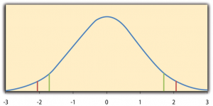
Fortunately, we do not have to deal directly with the distribution of  t  scores. If we were to enter our sample data and hypothetical mean of interest into one of the online statistical tools in Chapter 12 or into a program like SPSS (Excel does not have a one-sample  t- test function), the output would include both the  t  score and the  p  value. At this point, the rest of the procedure is simple. If  p  is equal to or less than .05, we reject the null hypothesis and conclude that the population mean differs from the hypothetical mean of interest. If  p  is greater than .05, we retain the null hypothesis and conclude that there is not enough evidence to say that the population mean differs from the hypothetical mean of interest. (Again, technically, we conclude only that we do not have enough evidence to conclude that it  does  differ.)

If we were to compute the  t  score by hand, we could use a table like Table 13.2 to make the decision. This table does not provide actual  p  values. Instead, it provides the  critical values  of  t  for different degrees of freedom ( df)  when α is .05. For now, let us focus on the two-tailed critical values in the last column of the table. Each of these values should be interpreted as a pair of values: one positive and one negative. For example, the two-tailed critical values when there are 24 degrees of freedom are 2.064 and −2.064. These are represented by the red vertical lines in Figure 13.1. The idea is that any  t  score below the lower critical value (the left-hand red line in Figure 13.1) is in the lowest 2.5% of the distribution, while any  t  score above the upper critical value (the right-hand red line) is in the highest 2.5% of the distribution. Therefore any  t  score beyond the critical value in  either  direction is in the most extreme 5% of  t  scores when the null hypothesis is true and has a  p  value less than .05. Thus if the  t  score we compute is beyond the critical value in either direction, then we reject the null hypothesis. If the  t  score we compute is between the upper and lower critical values, then we retain the null hypothesis.

Thus far, we have considered what is called a  two-tailed test , where we reject the null hypothesis if the  t  score for the sample is extreme in either direction. This test makes sense when we believe that the sample mean might differ from the hypothetical population mean but we do not have good reason to expect the difference to go in a particular direction. But it is also possible to do a  one-tailed test , where we reject the null hypothesis only if the  t  score for the sample is extreme in one direction that we specify before collecting the data. This test makes sense when we have good reason to expect the sample mean will differ from the hypothetical population mean in a particular direction.

Here is how it works. Each one-tailed critical value in Table 13.2 can again be interpreted as a pair of values: one positive and one negative. A  t  score below the lower critical value is in the lowest 5% of the distribution, and a  t  score above the upper critical value is in the highest 5% of the distribution. For 24 degrees of freedom, these values are −1.711 and 1.711. (These are represented by the green vertical lines in Figure 13.1.) However, for a one-tailed test, we must decide before collecting data whether we expect the sample mean to be lower than the hypothetical population mean, in which case we would use only the lower critical value, or we expect the sample mean to be greater than the hypothetical population mean, in which case we would use only the upper critical value. Notice that we still reject the null hypothesis when the  t  score for our sample is in the most extreme 5% of the t scores we would expect if the null hypothesis were true—so α remains at .05. We have simply redefined  extreme  to refer only to one tail of the distribution. The advantage of the one-tailed test is that critical values are less extreme. If the sample mean differs from the hypothetical population mean in the expected direction, then we have a better chance of rejecting the null hypothesis. The disadvantage is that if the sample mean differs from the hypothetical population mean in the unexpected direction, then there is no chance at all of rejecting the null hypothesis.

Example One-Sample  t – Test

Imagine that a health psychologist is interested in the accuracy of university students’ estimates of the number of calories in a chocolate chip cookie. He shows the cookie to a sample of 10 students and asks each one to estimate the number of calories in it. Because the actual number of calories in the cookie is 250, this is the hypothetical population mean of interest (µ 0 ). The null hypothesis is that the mean estimate for the population (μ) is 250. Because he has no real sense of whether the students will underestimate or overestimate the number of calories, he decides to do a two-tailed test. Now imagine further that the participants’ actual estimates are as follows:

250, 280, 200, 150, 175, 200, 200, 220, 180, 250.

The mean estimate for the sample ( M ) is 212.00 calories and the standard deviation ( SD ) is 39.17. The health psychologist can now compute the  t  score for his sample:

[latex]t=\dfrac{{212-250}}{\left(\dfrac{39.17}{\sqrt10}\right)}=-3.07[/latex]

If he enters the data into one of the online analysis tools or uses SPSS, it would also tell him that the two-tailed p  value for this  t  score (with 10 − 1 = 9 degrees of freedom) is .013. Because this is less than .05, the health psychologist would reject the null hypothesis and conclude that university students tend to underestimate the number of calories in a chocolate chip cookie. If he computes the  t  score by hand, he could look at Table 13.2 and see that the critical value of  t  for a two-tailed test with 9 degrees of freedom is ±2.262. The fact that his  t  score was more extreme than this critical value would tell him that his  p  value is less than .05 and that he should reject the null hypothesis. Using APA style, these results would be reported as follows:  t (9) = -3.07,  p  = .01. Note that the  t  and  p  are italicized, the degrees of freedom appear in brackets with no decimal remainder, and the values of  t  and  p  are rounded to two decimal places.

Finally, if this researcher had gone into this study with good reason to expect that university students underestimate the number of calories, then he could have done a one-tailed test instead of a two-tailed test. The only thing this decision would change is the critical value, which would be −1.833. This slightly less extreme value would make it a bit easier to reject the null hypothesis. However, if it turned out that university students overestimate the number of calories—no matter how much they overestimate it—the researcher would not have been able to reject the null hypothesis.

The Dependent-Samples  t – Test

The  dependent-samples  t -test  (sometimes called the paired-samples  t- test) is used to compare two means for the same sample tested at two different times or under two different conditions. This comparison is appropriate for pretest-posttest designs or within-subjects experiments. The null hypothesis is that the means at the two times or under the two conditions are the same in the population. The alternative hypothesis is that they are not the same. This test can also be one-tailed if the researcher has good reason to expect the difference goes in a particular direction.

It helps to think of the dependent-samples  t- test as a special case of the one-sample  t- test. However, the first step in the dependent-samples  t- test is to reduce the two scores for each participant to a single  difference score  by taking the difference between them. At this point, the dependent-samples  t- test becomes a one-sample  t- test on the difference scores. The hypothetical population mean (µ 0 ) of interest is 0 because this is what the mean difference score would be if there were no difference on average between the two times or two conditions. We can now think of the null hypothesis as being that the mean difference score in the population is 0 (µ 0  = 0) and the alternative hypothesis as being that the mean difference score in the population is not 0 (µ 0  ≠ 0).

Example Dependent-Samples  t – Test

Imagine that the health psychologist now knows that people tend to underestimate the number of calories in junk food and has developed a short training program to improve their estimates. To test the effectiveness of this program, he conducts a pretest-posttest study in which 10 participants estimate the number of calories in a chocolate chip cookie before the training program and then again afterward. Because he expects the program to increase the participants’ estimates, he decides to do a one-tailed test. Now imagine further that the pretest estimates are

230, 250, 280, 175, 150, 200, 180, 210, 220, 190

and that the posttest estimates (for the same participants in the same order) are

250, 260, 250, 200, 160, 200, 200, 180, 230, 240.

The difference scores, then, are as follows:

20, 10, −30, 25, 10, 0, 20, −30, 10, 50.

Note that it does not matter whether the first set of scores is subtracted from the second or the second from the first as long as it is done the same way for all participants. In this example, it makes sense to subtract the pretest estimates from the posttest estimates so that positive difference scores mean that the estimates went up after the training and negative difference scores mean the estimates went down.

The mean of the difference scores is 8.50 with a standard deviation of 27.27. The health psychologist can now compute the  t  score for his sample as follows:

[latex]t=\dfrac{{8.5-0}}{\left(\dfrac{27.27}{\sqrt10}\right)}=1.11[/latex]

If he enters the data into one of the online analysis tools or uses Excel or SPSS, it would tell him that the one-tailed  p  value for this  t  score (again with 10 − 1 = 9 degrees of freedom) is .148. Because this is greater than .05, he would retain the null hypothesis and conclude that the training program does not significantly increase people’s calorie estimates. If he were to compute the  t  score by hand, he could look at Table 13.2 and see that the critical value of  t for a one-tailed test with 9 degrees of freedom is 1.833. (It is positive this time because he was expecting a positive mean difference score.) The fact that his  t score was less extreme than this critical value would tell him that his  p  value is greater than .05 and that he should fail to reject the null hypothesis.

The Independent-Samples  t- Test

The  independent-samples  t- test  is used to compare the means of two separate samples ( M 1  and  M 2 ). The two samples might have been tested under different conditions in a between-subjects experiment, or they could be pre-existing groups in a cross-sectional design (e.g., women and men, extraverts and introverts). The null hypothesis is that the means of the two populations are the same: µ 1  = µ 2 . The alternative hypothesis is that they are not the same: µ 1  ≠ µ 2 . Again, the test can be one-tailed if the researcher has good reason to expect the difference goes in a particular direction.

The  t  statistic here is a bit more complicated because it must take into account two sample means, two standard deviations, and two sample sizes. The formula is as follows:

[latex]t=\dfrac{{M{_1}-M{_2}}}{\sqrt{\dfrac{SD{^2}{_1}}{n{_1}}+\dfrac{SD{^2}{_2}}{n{_2}}}}[/latex]

Notice that this formula includes squared standard deviations (the variances) that appear inside the square root symbol. Also, lowercase  n 1  and  n 2  refer to the sample sizes in the two groups or condition (as opposed to capital  N , which generally refers to the total sample size). The only additional thing to know here is that there are  N  − 2 degrees of freedom for the independent-samples  t-  test.

Example Independent-Samples  t – Test

Now the health psychologist wants to compare the calorie estimates of people who regularly eat junk food with the estimates of people who rarely eat junk food. He believes the difference could come out in either direction so he decides to conduct a two-tailed test. He collects data from a sample of eight participants who eat junk food regularly and seven participants who rarely eat junk food. The data are as follows:

Junk food eaters: 180, 220, 150, 85, 200, 170, 150, 190

Non–junk food eaters: 200, 240, 190, 175, 200, 300, 240

The mean for the non-junk food eaters is 220.71 with a standard deviation of 41.23. The mean for the junk food eaters is 168.12 with a standard deviation of 42.66. He can now compute his  t  score as follows:

[latex]t=\dfrac{{220.71-168.12}}{\sqrt{\dfrac{41.23{^2}}{8}+\dfrac{42.66{^2}}{7}}}= 2.42[/latex]

If he enters the data into one of the online analysis tools or uses Excel or SPSS, it would tell him that the two-tailed  p  value for this  t  score (with 15 − 2 = 13 degrees of freedom) is .015. Because this p value is less than .05, the health psychologist would reject the null hypothesis and conclude that people who eat junk food regularly make lower calorie estimates than people who eat it rarely. If he were to compute the  t  score by hand, he could look at Table 13.2 and see that the critical value of  t  for a two-tailed test with 13 degrees of freedom is ±2.160. The fact that his  t  score was more extreme than this critical value would tell him that his  p  value is less than .05 and that he should reject the null hypothesis.

The Analysis of Variance

T -tests are used to compare two means (a sample mean with a population mean, the means of two conditions or two groups). When there are more than two groups or condition means to be compared, the most common null hypothesis test is the  analysis of variance (ANOVA) . In this section, we look primarily at the  one-way ANOVA , which is used for between-subjects designs with a single independent variable. We then briefly consider some other versions of the ANOVA that are used for within-subjects and factorial research designs.

One-Way ANOVA

The one-way ANOVA is used to compare the means of more than two samples ( M 1 ,  M 2 … M G ) in a between-subjects design. The null hypothesis is that all the means are equal in the population: µ 1 = µ 2  =…= µ G . The alternative hypothesis is that not all the means in the population are equal.

The test statistic for the ANOVA is called  F . It is a ratio of two estimates of the population variance based on the sample data. One estimate of the population variance is called the  mean squares between groups (MS B )  and is based on the differences among the sample means. The other is called the mean squares within groups (MS W )  and is based on the differences among the scores within each group. The  F  statistic is the ratio of the  MS B  to the  MS W and can, therefore, be expressed as follows:

F = MS B / MS W

Again, the reason that  F  is useful is that we know how it is distributed when the null hypothesis is true. As shown in Figure 13.2, this distribution is unimodal and positively skewed with values that cluster around 1. The precise shape of the distribution depends on both the number of groups and the sample size, and there are degrees of freedom values associated with each of these. The between-groups degrees of freedom is the number of groups minus one:  df B  = ( G  − 1). The within-groups degrees of freedom is the total sample size minus the number of groups:  df W  =  N  −  G . Again, knowing the distribution of  F when the null hypothesis is true allows us to find the  p  value.

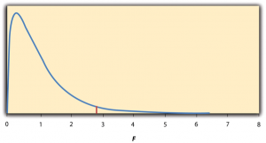
The online tools in Chapter 12 and statistical software such as Excel and SPSS will compute  F  and find the  p  value. If  p  is equal to or less than .05, then we reject the null hypothesis and conclude that there are differences among the group means in the population. If  p  is greater than .05, then we retain the null hypothesis and conclude that there is not enough evidence to say that there are differences. In the unlikely event that we would compute  F  by hand, we can use a table of critical values like Table 13.3 “Table of Critical Values of ” to make the decision. The idea is that any  F  ratio greater than the critical value has a  p value of less than .05. Thus if the  F  ratio we compute is beyond the critical value, then we reject the null hypothesis. If the F ratio we compute is less than the critical value, then we retain the null hypothesis.

Example One-Way ANOVA

Imagine that the health psychologist wants to compare the calorie estimates of psychology majors, nutrition majors, and professional dieticians. He collects the following data:

Psych majors: 200, 180, 220, 160, 150, 200, 190, 200

Nutrition majors: 190, 220, 200, 230, 160, 150, 200, 210, 195

Dieticians: 220, 250, 240, 275, 250, 230, 200, 240

The means are 187.50 ( SD  = 23.14), 195.00 ( SD  = 27.77), and 238.13 ( SD  = 22.35), respectively. So it appears that dieticians made substantially more accurate estimates on average. The researcher would almost certainly enter these data into a program such as Excel or SPSS, which would compute  F  for him or her and find the  p  value. Table 13.4 shows the output of the one-way ANOVA function in Excel for these data. This table is referred to as an ANOVA table. It shows that  MS B  is 5,971.88,  MS W  is 602.23, and their ratio,  F , is 9.92. The  p  value is .0009. Because this value is below .05, the researcher would reject the null hypothesis and conclude that the mean calorie estimates for the three groups are not the same in the population. Notice that the ANOVA table also includes the “sum of squares” ( SS ) for between groups and for within groups. These values are computed on the way to finding  MS B  and MS W  but are not typically reported by the researcher. Finally, if the researcher were to compute the  F  ratio by hand, he could look at Table 13.3 and see that the critical value of  F  with 2 and 21 degrees of freedom is 3.467 (the same value in Table 13.4 under  F crit ). The fact that his  F  score was more extreme than this critical value would tell him that his  p  value is less than .05 and that he should reject the null hypothesis.

ANOVA Elaborations

Post hoc comparisons.

When we reject the null hypothesis in a one-way ANOVA, we conclude that the group means are not all the same in the population. But this can indicate different things. With three groups, it can indicate that all three means are significantly different from each other. Or it can indicate that one of the means is significantly different from the other two, but the other two are not significantly different from each other. It could be, for example, that the mean calorie estimates of psychology majors, nutrition majors, and dieticians are all significantly different from each other. Or it could be that the mean for dieticians is significantly different from the means for psychology and nutrition majors, but the means for psychology and nutrition majors are not significantly different from each other. For this reason, statistically significant one-way ANOVA results are typically followed up with a series of  post hoc comparisons  of selected pairs of group means to determine which are different from which others.

One approach to post hoc comparisons would be to conduct a series of independent-samples  t- tests comparing each group mean to each of the other group means. But there is a problem with this approach. In general, if we conduct a  t -test when the null hypothesis is true, we have a 5% chance of mistakenly rejecting the null hypothesis (see Section 13.3 “Additional Considerations” for more on such Type I errors). If we conduct several  t- tests when the null hypothesis is true, the chance of mistakenly rejecting  at least one null hypothesis increases with each test we conduct. Thus researchers do not usually make post hoc comparisons using standard  t- tests because there is too great a chance that they will mistakenly reject at least one null hypothesis. Instead, they use one of several modified  t -test procedures—among them the Bonferonni procedure, Fisher’s least significant difference (LSD) test, and Tukey’s honestly significant difference (HSD) test. The details of these approaches are beyond the scope of this book, but it is important to understand their purpose. It is to keep the risk of mistakenly rejecting a true null hypothesis to an acceptable level (close to 5%).

Repeated-Measures ANOVA

Recall that the one-way ANOVA is appropriate for between-subjects designs in which the means being compared come from separate groups of participants. It is not appropriate for within-subjects designs in which the means being compared come from the same participants tested under different conditions or at different times. This requires a slightly different approach, called the repeated-measures ANOVA . The basics of the repeated-measures ANOVA are the same as for the one-way ANOVA. The main difference is that measuring the dependent variable multiple times for each participant allows for a more refined measure of  MS W . Imagine, for example, that the dependent variable in a study is a measure of reaction time. Some participants will be faster or slower than others because of stable individual differences in their nervous systems, muscles, and other factors. In a between-subjects design, these stable individual differences would simply add to the variability within the groups and increase the value of  MS W (which would, in turn, decrease the value of F). In a within-subjects design, however, these stable individual differences can be measured and subtracted from the value of  MS W . This lower value of  MS W  means a higher value of  F  and a more sensitive test.

Factorial ANOVA

When more than one independent variable is included in a factorial design, the appropriate approach is the  factorial ANOVA . Again, the basics of the factorial ANOVA are the same as for the one-way and repeated-measures ANOVAs. The main difference is that it produces an  F  ratio and  p  value for each main effect and for each interaction. Returning to our calorie estimation example, imagine that the health psychologist tests the effect of participant major (psychology vs. nutrition) and food type (cookie vs. hamburger) in a factorial design. A factorial ANOVA would produce separate  F  ratios and  p values for the main effect of major, the main effect of food type, and the interaction between major and food. Appropriate modifications must be made depending on whether the design is between-subjects, within-subjects, or mixed.

Testing Correlation Coefficients

For relationships between quantitative variables, where Pearson’s  r (the correlation coefficient)   is used to describe the strength of those relationships, the appropriate null hypothesis test is a test of the correlation coefficient. The basic logic is exactly the same as for other null hypothesis tests. In this case, the null hypothesis is that there is no relationship in the population. We can use the Greek lowercase rho (ρ) to represent the relevant parameter: ρ = 0. The alternative hypothesis is that there is a relationship in the population: ρ ≠ 0. As with the  t-  test, this test can be two-tailed if the researcher has no expectation about the direction of the relationship or one-tailed if the researcher expects the relationship to go in a particular direction.

It is possible to use the correlation coefficient for the sample to compute a  t  score with  N  − 2 degrees of freedom and then to proceed as for a  t- test. However, because of the way it is computed, the correlation coefficient can also be treated as its own test statistic. The online statistical tools and statistical software such as Excel and SPSS generally compute the correlation coefficient and provide the  p  value associated with that value. As always, if the  p  value is equal to or less than .05, we reject the null hypothesis and conclude that there is a relationship between the variables in the population. If the  p  value is greater than .05, we retain the null hypothesis and conclude that there is not enough evidence to say there is a relationship in the population. If we compute the correlation coefficient by hand, we can use a table like Table 13.5, which shows the critical values of  r  for various samples sizes when α is .05. A sample value of the correlation coefficient that is more extreme than the critical value is statistically significant.

Example Test of a Correlation Coefficient

Imagine that the health psychologist is interested in the correlation between people’s calorie estimates and their weight. She has no expectation about the direction of the relationship, so she decides to conduct a two-tailed test. She computes the correlation coefficient for a sample of 22 university students and finds that Pearson’s  r  is −.21. The statistical software she uses tells her that the  p  value is .348. It is greater than .05, so she retains the null hypothesis and concludes that there is no relationship between people’s calorie estimates and their weight. If she were to compute the correlation coefficient by hand, she could look at Table 13.5 and see that the critical value for 22 − 2 = 20 degrees of freedom is .444. The fact that the correlation coefficient for her sample is less extreme than this critical value tells her that the  p  value is greater than .05 and that she should retain the null hypothesis.

A test that involves looking at the difference between two means.

Used to compare a sample mean (M) with a hypothetical population mean (μ0) that provides some interesting standard of comparison.

A statistic (e.g., F , t , etc.) that is computed to compare against what is expected in the null hypothesis, and thus helps find the p value.

The absolute value that a test statistic (e.g., F , t , etc.) must exceed to be considered statistically significant.

Where we reject the null hypothesis if the test statistic for the sample is extreme in either direction (+/-).

Where we reject the null hypothesis only if the  t  score for the sample is extreme in one direction that we specify before collecting the data.

Used to compare two means for the same sample tested at two different times or under two different conditions (sometimes called the paired-samples  t -test).

A method to reduce pairs of scores (e.g., pre- and post-test) to a single score by calculating the difference between them.

Used to compare the means of two separate samples (M1 and M2).

A statistical test used when there are more than two groups or condition means to be compared.

Used for between-subjects designs with a single independent variable.

An estimate of the population variance and is based on the differences among the sample means.

An estimate of the population variance and is based on the differences among the scores within each group.

An unplanned (not hypothesized) test of which pairs of group mean scores are different from which others.

Compares the means from the same participants tested under different conditions or at different times in which the dependent variable is measured multiple times for each participant.

A statistical method to detect differences in the means between conditions when there are two or more independent variables in a factorial design. It allows the detection of main effects and interaction effects.

Research Methods in Psychology Copyright © 2019 by Rajiv S. Jhangiani, I-Chant A. Chiang, Carrie Cuttler, & Dana C. Leighton is licensed under a Creative Commons Attribution-NonCommercial-ShareAlike 4.0 International License , except where otherwise noted.

Share This Book