presentation in global warming

Climate Matters • November 25, 2020

New Presentation: Our Changing Climate

Key concepts:.

Climate Central unveils Our Changing Climate —an informative and customizable climate change presentation that meteorologists, journalists, and others can use for educational outreach and/or a personal Climate 101 tool.

The presentation follows a ”Simple, Serious, Solvable” framework, inspired by climate scientist Scott Denning. This allows the presenter to comfortably explain, and the viewers to easily understand, the causes (Simple), impacts (Serious), and solutions (Solvable) of climate change. 

Our Changing Climate is a revamped version of our 2016 climate presentation, and includes the following updates and features:

Up-to-date graphics and topics

Local data and graphics

Fully editable slides (add, remove, customize)

Presenter notes, background information, and references for each slide

Supplementary and bonus slides

Download Outline (PDF, 110KB)

Download Full Presentation (PPT, 148MB)

Updated: April 2021

Climate Central is presenting a new outreach and education resource for meteorologists, journalists, and others—a climate change presentation, Our Changing Climate . This 55-slide presentation is a guide through the basics of climate change, outlining its causes, impacts, and solutions. This climate change overview is unique because it includes an array of local graphics from our ever-expanding media library. By providing these local angles, the presenter can demonstrate that climate change is not only happening at a global-scale, but in our backyards.

This presentation was designed to support your climate change storytelling, but can also double as a great Climate 101 tool for journalists or educators who want to understand climate change better. Every slide contains main points along with background information, so people that are interested can learn at their own pace or utilize graphics for their own content. 

In addition to those features, it follows the “Simple, Serious, Solvable” framework inspired by Scott Denning, a climate scientist and professor of atmospheric science at Colorado State University (and a good friend of the program). These three S’s help create the presentation storyline and outline the causes (Simple), impacts (Serious), and solutions (Solvable) of climate change. 

Simple. It is simple—burning fossil fuels is heating up the Earth. This section outlines the well-understood science that goes back to the 1800s, presenting local and global evidence that our climate is warming due to human activities.

Serious. More extreme weather, rising sea levels, and increased health and economic risks—the consequences of climate change. In this section, well, we get serious. Climate change impacts are already being felt around the world, and they will continue to intensify until we cut greenhouse gas emissions. 

Solvable. With such a daunting crisis like climate change, it is easy to get wrapped up in the negative impacts. This section explains how we can curb climate change and lists the main pathways and solutions to achieving this goal. 

With the rollout of our new climate change presentation, we at Climate Central would value any feedback on this presentation. Feel free to reach out to us about how the presentation worked for you, how your audience reacted, or any ideas or topics you would like to see included. 

ACKNOWLEDGMENTS & SPECIAL THANKS

Climate Central would like to acknowledge Paul Gross at WDIV-TV in Detroit and the AMS Station Science Committee for the original version of the climate presentation, Climate Change Outreach Presentation , that was created in 2016. We would also like to give special thanks to Scott Denning, professor of atmospheric science at Colorado State University and a member of our NSF advisory board, for allowing us to use this “Simple, Serious, Solvable” framework in this presentation resource.

SUPPORTING MULTIMEDIA

ENCYCLOPEDIC ENTRY

Global warming.

The causes, effects, and complexities of global warming are important to understand so that we can fight for the health of our planet.

Earth Science, Climatology

Tennessee Power Plant

Ash spews from a coal-fueled power plant in New Johnsonville, Tennessee, United States.

Photograph by Emory Kristof/ National Geographic

Global warming is the long-term warming of the planet’s overall temperature. Though this warming trend has been going on for a long time, its pace has significantly increased in the last hundred years due to the burning of fossil fuels . As the human population has increased, so has the volume of fossil fuels burned. Fossil fuels include coal, oil, and natural gas, and burning them causes what is known as the “greenhouse effect” in Earth’s atmosphere.

The greenhouse effect is when the sun’s rays penetrate the atmosphere, but when that heat is reflected off the surface cannot escape back into space. Gases produced by the burning of fossil fuels prevent the heat from leaving the atmosphere. These greenhouse gasses are carbon dioxide , chlorofluorocarbons, water vapor , methane , and nitrous oxide . The excess heat in the atmosphere has caused the average global temperature to rise overtime, otherwise known as global warming.

Global warming has presented another issue called climate change. Sometimes these phrases are used interchangeably, however, they are different. Climate change refers to changes in weather patterns and growing seasons around the world. It also refers to sea level rise caused by the expansion of warmer seas and melting ice sheets and glaciers . Global warming causes climate change, which poses a serious threat to life on Earth in the forms of widespread flooding and extreme weather. Scientists continue to study global warming and its impact on Earth.

Media Credits

The audio, illustrations, photos, and videos are credited beneath the media asset, except for promotional images, which generally link to another page that contains the media credit. The Rights Holder for media is the person or group credited.

Production Managers

Program specialists, last updated.

February 21, 2024

User Permissions

For information on user permissions, please read our Terms of Service. If you have questions about how to cite anything on our website in your project or classroom presentation, please contact your teacher. They will best know the preferred format. When you reach out to them, you will need the page title, URL, and the date you accessed the resource.

If a media asset is downloadable, a download button appears in the corner of the media viewer. If no button appears, you cannot download or save the media.

Text on this page is printable and can be used according to our Terms of Service .

Interactives

Any interactives on this page can only be played while you are visiting our website. You cannot download interactives.

Related Resources

Global Climate Change

By: Neill Chua & Patrick Moraitis

What is Climate Change?

• The gradual increase in the global temperature.
• Natural events and human activities are believed to be contributing to an increase in average global temperatures.
• This is caused primarily by increases in “greenhouse” gases such as Carbon Dioxide (CO 2 )

Greenhouse Gases

• Temperature of the Earth is determined by the balance between the input from energy from the Sun and the reflection of some of this energy back into space
• Greenhouse Gases trap some of the heat reflected back to the sun
• Massive increase in recent years due to Global Warming

Causes of Climate Change

• Burning of Fossil fuels
• ⅘ of global carbon dioxide emissions come from energy production, transport, and industrial processes
• Emissions not equal around the world
• More developed countries produce much more
• North America, Europe, Asia

Causes of Climate Change cont.

• Land Use Changes
• Ex: deforestation for the purposes of agriculture, urbanization, or roads
• Happens more in developing countries
• Most developed countries did this in the industrial revolution

What can be done?

• Target major research universities to help find better ways to go into developing cheap and clean energy production, as all economic development is based on increasing energy usage
• $1 trillion spent on Iraq war, but only $1 billion going into global warming issues
• Increase on developing “Renewable Energy Sources”
• Reduce the waste of energy being spent on the development of society

Interactive Data Visualization

• Highlights key locations around the world and visualizes how much its current temperature deviates from historical averages or records for the current day
• Uses symbols and color to represent data which can be clicked for data summary
• Uses up to the minute live data from Weather Underground API
• Key locations include:
• ~50 of thee most populated cities & major world cities
• ~15 places with the lowest recorded temperatures on earth (-30F & below)
• ~15 places with the highest recorded temperatures on earth (100F & above)
• Our main audience ranges from everyday people who have an interest in Global Climate Change to the expert scientific research community.
• We want people to use this project as a springboard to begin engaging with the global warming phenomenon in a subjective environment.
• Primarily raw data presented in a digestible way that isn’t biased, allowing people to create their own ideas on this pressing global social issue
• Eventually, we want to be able to implement our project to bigger corporations or even the government in helping aid with understanding which areas around the world have the biggest climate change problems.

Data Visualization Iterations

We explored several map libraries, weather data APIs, and more.

You can see our detailed preliminary progress reports here

• http://nc-data-visualization.tumblr.com/post/134924457119/final-project-email &
• http://patrickmoraitis.blogspot.com/2015/12/data-visualization-post-9-final-project.html

How did we make it?

• Cesium, an open-source JS library for 3D maps
• Google sheets to store location data and create feeds
• Weather Underground API for current temperature and almanac data
• Add historical weather data to show long term trends (but this is not as easy/affordable to obtain as current data)
• Possibly save multiple days’ worth of data, and show in a different visualization how the weather changes over a period of day and whether that period of time still has a regular deviation.
• Add more & refine current locations, but no more than 99 due to API limits
• Allow user to enter and retrieve weather data for custom location
• Open source to developer community and get expert data & weather scientists involved

What Is Climate Change?

Climate change is a long-term change in the average weather patterns that have come to define Earth’s local, regional and global climates. These changes have a broad range of observed effects that are synonymous with the term.

Changes observed in Earth’s climate since the mid-20th century are driven by human activities, particularly fossil fuel burning, which increases heat-trapping greenhouse gas levels in Earth’s atmosphere, raising Earth’s average surface temperature. Natural processes, which have been overwhelmed by human activities, can also contribute to climate change, including internal variability (e.g., cyclical ocean patterns like El Niño, La Niña and the Pacific Decadal Oscillation) and external forcings (e.g., volcanic activity, changes in the Sun’s energy output , variations in Earth’s orbit ).

Scientists use observations from the ground, air, and space, along with computer models , to monitor and study past, present, and future climate change. Climate data records provide evidence of climate change key indicators, such as global land and ocean temperature increases; rising sea levels; ice loss at Earth’s poles and in mountain glaciers; frequency and severity changes in extreme weather such as hurricanes, heatwaves, wildfires, droughts, floods, and precipitation; and cloud and vegetation cover changes.

“Climate change” and “global warming” are often used interchangeably but have distinct meanings. Similarly, the terms "weather" and "climate" are sometimes confused, though they refer to events with broadly different spatial- and timescales.

What Is Global Warming?

Global warming is the long-term heating of Earth’s surface observed since the pre-industrial period (between 1850 and 1900) due to human activities, primarily fossil fuel burning, which increases heat-trapping greenhouse gas levels in Earth’s atmosphere. This term is not interchangeable with the term "climate change."

Since the pre-industrial period, human activities are estimated to have increased Earth’s global average temperature by about 1 degree Celsius (1.8 degrees Fahrenheit), a number that is currently increasing by more than 0.2 degrees Celsius (0.36 degrees Fahrenheit) per decade. The current warming trend is unequivocally the result of human activity since the 1950s and is proceeding at an unprecedented rate over millennia.

Weather vs. Climate

“if you don’t like the weather in new england, just wait a few minutes.” - mark twain.

Weather refers to atmospheric conditions that occur locally over short periods of time—from minutes to hours or days. Familiar examples include rain, snow, clouds, winds, floods, or thunderstorms.

Climate, on the other hand, refers to the long-term (usually at least 30 years) regional or even global average of temperature, humidity, and rainfall patterns over seasons, years, or decades.

Find Out More: A Guide to NASA’s Global Climate Change Website

This website provides a high-level overview of some of the known causes, effects and indications of global climate change:

Evidence. Brief descriptions of some of the key scientific observations that our planet is undergoing abrupt climate change.

Causes. A concise discussion of the primary climate change causes on our planet.

Effects. A look at some of the likely future effects of climate change, including U.S. regional effects.

Vital Signs. Graphs and animated time series showing real-time climate change data, including atmospheric carbon dioxide, global temperature, sea ice extent, and ice sheet volume.

Earth Minute. This fun video series explains various Earth science topics, including some climate change topics.

Other NASA Resources

Goddard Scientific Visualization Studio. An extensive collection of animated climate change and Earth science visualizations.

Sea Level Change Portal. NASA's portal for an in-depth look at the science behind sea level change.

NASA’s Earth Observatory. Satellite imagery, feature articles and scientific information about our home planet, with a focus on Earth’s climate and environmental change.

Header image is of Apusiaajik Glacier, and was taken near Kulusuk, Greenland, on Aug. 26, 2018, during NASA's Oceans Melting Greenland (OMG) field operations. Learn more here . Credit: NASA/JPL-Caltech

Discover More Topics From NASA

Explore Earth Science

Earth Science in Action

Earth Science Data

Facts About Earth

• ENVIRONMENT

How global warming is disrupting life on Earth

The signs of global warming are everywhere, and are more complex than just climbing temperatures.

Our planet is getting hotter. Since the Industrial Revolution—an event that spurred the use of fossil fuels in everything from power plants to transportation—Earth has warmed by 1 degree Celsius, about 2 degrees Fahrenheit.  

That may sound insignificant, but 2023 was the hottest year on record , and all 10 of the hottest years on record have occurred in the past decade.  

Global warming and climate change are often used interchangeably as synonyms, but scientists prefer to use “climate change” when describing the complex shifts now affecting our planet’s weather and climate systems.  

Climate change encompasses not only rising average temperatures but also natural disasters, shifting wildlife habitats, rising seas , and a range of other impacts. All of these changes are emerging as humans continue to add heat-trapping greenhouse gases , like carbon dioxide and methane, to the atmosphere.

What causes global warming?

When fossil fuel emissions are pumped into the atmosphere, they change the chemistry of our atmosphere, allowing sunlight to reach the Earth but preventing heat from being released into space. This keeps Earth warm, like a greenhouse, and this warming is known as the greenhouse effect .  

Carbon dioxide is the most commonly found greenhouse gas and about 75 percent of all the climate warming pollution in the atmosphere. This gas is a product of producing and burning oil, gas, and coal. About a quarter of Carbon dioxide also results from land cleared for timber or agriculture.  

Methane is another common greenhouse gas. Although it makes up only about 16 percent of emissions, it's roughly 25 times more potent than carbon dioxide and dissipates more quickly. That means methane can cause a large spark in warming, but ending methane pollution can also quickly limit the amount of atmospheric warming. Sources of this gas include agriculture (mostly livestock), leaks from oil and gas production, and waste from landfills.  

What are the effects of global warming?  

One of the most concerning impacts of global warming is the effect warmer temperatures will have on Earth's polar regions and mountain glaciers. The Arctic is warming four times faster than the rest of the planet. This warming reduces critical ice habitat and it disrupts the flow of the jet stream, creating more unpredictable weather patterns around the globe.  

( Learn more about the jet stream. )

A warmer planet doesn't just raise temperatures. Precipitation is becoming more extreme as the planet heats. For every degree your thermometer rises, the air holds about seven percent more moisture. This increase in moisture in the atmosphere can produce flash floods, more destructive hurricanes, and even paradoxically, stronger snow storms.  

The world's leading scientists regularly gather to review the latest research on how the planet is changing. The results of this review is synthesized in regularly published reports known as the Intergovernmental Panel on Climate Change (IPCC) reports.  

A recent report outlines how disruptive a global rise in temperature can be:

• Coral reefs are now a highly endangered ecosystem. When corals face environmental stress, such as high heat, they expel their colorful algae and turn a ghostly white, an effect known as coral bleaching . In this weakened state, they more easily die.  
• Trees are increasingly dying from drought , and this mass mortality is reshaping forest ecosystems.
• Rising temperatures and changing precipitation patterns are making wildfires more common and more widespread. Research shows they're even moving into the eastern U.S. where fires have historically been less common.
• Hurricanes are growing more destructive and dumping more rain, an effect that will result in more damage. Some scientists say we even need to be preparing for Cat 6 storms . (The current ranking system ends at Cat 5.)

How can we limit global warming?  

Limiting the rising in global warming is theoretically achievable, but politically, socially, and economically difficult.  

Those same sources of greenhouse gas emissions must be limited to reduce warming. For example, oil and gas used to generate electricity or power industrial manufacturing will need to be replaced by net zero emission technology like wind and solar power. Transportation, another major source of emissions, will need to integrate more electric vehicles, public transportation, and innovative urban design, such as safe bike lanes and walkable cities.  

( Learn more about solutions to limit global warming. )

One global warming solution that was once considered far fetched is now being taken more seriously: geoengineering. This type of technology relies on manipulating the Earth's atmosphere to physically block the warming rays of the sun or by sucking carbon dioxide straight out of the sky.

Restoring nature may also help limit warming. Trees, oceans, wetlands, and other ecosystems help absorb excess carbon—but when they're lost, so too is their potential to fight climate change.  

Ultimately, we'll need to adapt to warming temperatures, building homes to withstand sea level rise for example, or more efficiently cooling homes during heat waves.  

FREE BONUS ISSUE

Related topics.

• CLIMATE CHANGE
• ENVIRONMENT AND CONSERVATION
• POLAR REGIONS

You May Also Like

Why all life on Earth depends on trees

Life probably exists beyond Earth. So how do we find it?

For Antarctica’s emperor penguins, ‘there is no time left’

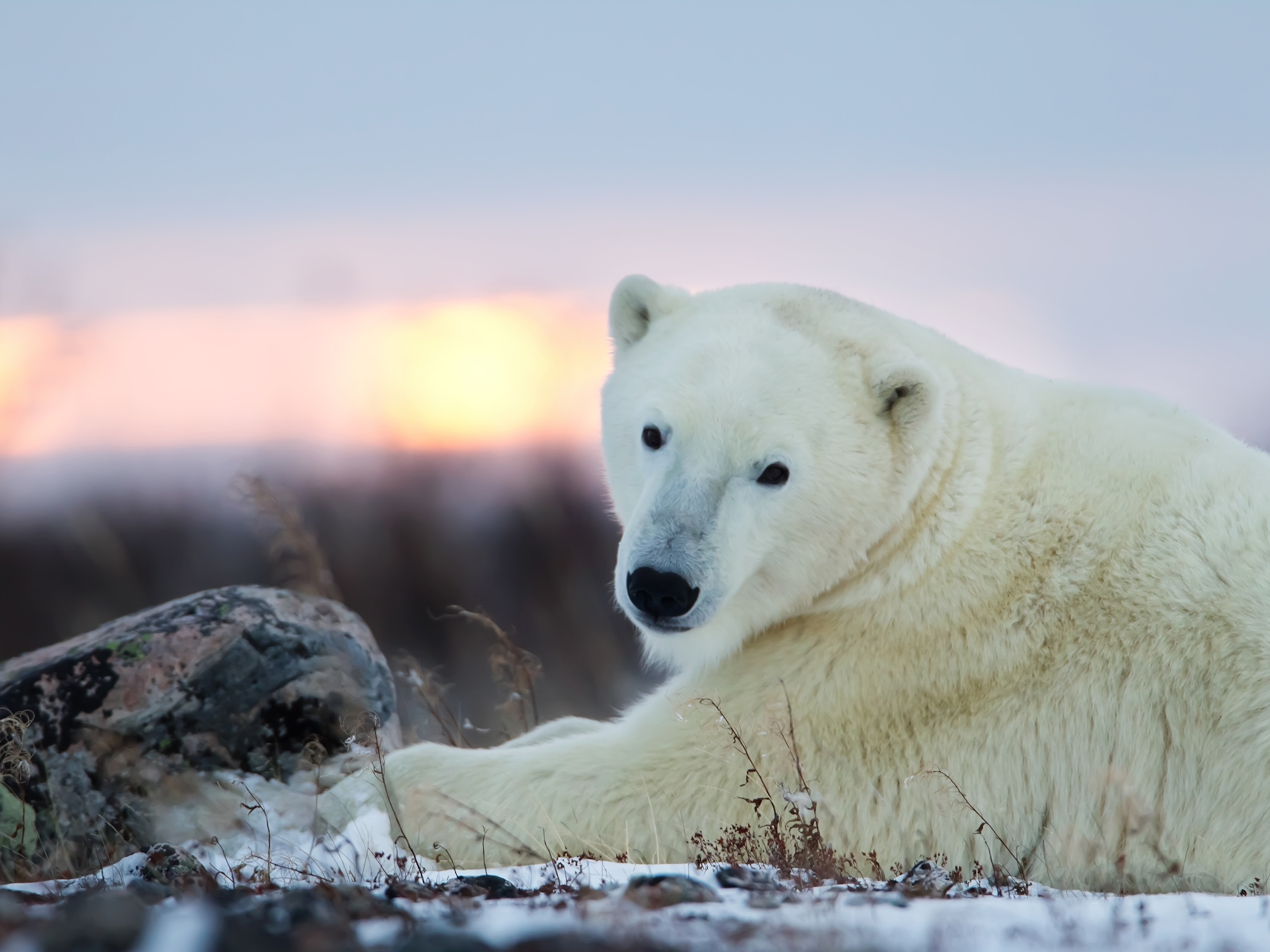
Polar bears are trying to adapt to a warming Arctic. It’s not working.

A photographic eulogy for Greenland's departing icebergs

• Environment
• Paid Content

History & Culture

• History & Culture
• History Magazine
• Gory Details
• 2023 in Review
• Mind, Body, Wonder
• Terms of Use
• Privacy Policy
• Your US State Privacy Rights
• Children's Online Privacy Policy
• Interest-Based Ads
• About Nielsen Measurement
• Do Not Sell or Share My Personal Information
• Nat Geo Home
• Attend a Live Event
• Book a Trip
• Inspire Your Kids
• Shop Nat Geo
• Visit the D.C. Museum
• Learn About Our Impact
• Support Our Mission
• Advertise With Us
• Customer Service
• Renew Subscription
• Manage Your Subscription
• Work at Nat Geo
• Sign Up for Our Newsletters
• Contribute to Protect the Planet

Copyright © 1996-2015 National Geographic Society Copyright © 2015-2024 National Geographic Partners, LLC. All rights reserved

Science News by AGU

Simpler Presentations of Climate Change

Share this:.

• Click to print (Opens in new window)
• Click to email a link to a friend (Opens in new window)
• Click to share on Twitter (Opens in new window)
• Click to share on Facebook (Opens in new window)
• Click to share on LinkedIn (Opens in new window)

Science Leads the Future

Are We Entering The Golden Age Of Climate Modeling?

Alumni push universities forward on climate, indoor air pollution in the time of coronavirus, how an unlikely friendship upended permafrost myths, the alarming rise of predatory conferences, science leads the future, and the future is now.

Has this happened to you? You are presenting the latest research about climate change to a general audience, maybe at the town library, to a local journalist, or even in an introductory science class. After presenting the solid science about greenhouse gases, how they work, and how we are changing them, you conclude with “and this is what the models predict about our climate future…”

At that point, your audience may feel they are being asked to make a leap of faith. Having no idea how the models work or what they contain and leave out, this final and crucial step becomes to them a “trust me” moment. Trust me moments can be easy to deny.

This problem has not been made easier by a recent expansion in the number of models and the range of predictions presented in the literature. One recent study making this point is that of Hausfather et al. [2022], which presents the “hot model” problem: the fact that some of the newer models in the Coupled Model Intercomparison Project Phase 6 (CMIP6) model comparison yield predictions of global temperatures that are above the range presented in the Intergovernmental Panel on Climate Change’s (IPCC) Sixth Assessment Report (AR6). The authors present a number of reasons for, and solutions to, the hot model problem.

Models are crucial in advancing any field of science. They represent a state-of-the-art summary of what the community understands about its subject. Differences among models highlight unknowns on which new research can be focused.

But Hausfather and colleagues make another point: As questions are answered and models evolve, they should also converge. That is, they should not only reproduce past measurements, but they should also begin to produce similar projections into the future. When that does not happen, it can make trust me moments even less convincing.

Are there simpler ways to make the major points about climate change, especially to general audiences, without relying on complex models?

We think there are.

Old Predictions That Still Hold True

In a recent article in Eos , Andrei Lapenis retells the story of Mikhail Budyko ’s 1972 predictions about global temperature and sea ice extent [ Budyko , 1972]. Lapenis notes that those predictions have proven to be remarkably accurate. This is a good example of effective, long-term predictions of climate change that are based on simple physical mechanisms that are relatively easy to explain.

There are many other examples that go back more than a century. These simpler formulations don’t attempt to capture the spatial or temporal detail of the full models, but their success at predicting the overall influence of rising carbon dioxide (CO 2 ) on global temperatures makes them a still-relevant, albeit mostly overlooked, resource in climate communication and even climate prediction.

One way to make use of this historical record is to present the relative consistency over time in estimates of equilibrium carbon sensitivity (ECS), the predicted change in mean global temperature expected from a doubling of atmospheric CO 2 . ECS can be presented in straightforward language, maybe even without the name and acronym, and is an understandable concept.

Estimates of ECS can be traced back for more than a century (Table 1), showing that the relationship between CO 2 in the atmosphere and Earth’s radiation and heat balance, as an expression of a simple and straightforward physical process, has been understood for a very long time. We can now measure that balance with precision [e.g., Loeb et al. , 2021], and measurements and modeling using improved technological expertise have all affirmed this scientific consistency.

Table 1. Selected Historical Estimates of Equilibrium Carbon Sensitivity (ECS)

Settled Science

Another approach for communicating with general audiences is to present an abbreviated history demonstrating that we have known the essentials of climate change for a very long time—that the basics are settled science.

The following list is a vastly oversimplified set of four milestones in the history of climate science that we have found to be effective. In a presentation setting, this four-step outline also provides a platform for a more detailed discussion if an audience wants to go there.

• 1850s: Eunice Foote observes that, when warmed by sunlight, a cylinder filled with CO 2 attained higher temperatures and cooled more slowly than one filled with ambient air, leading her to conclude that higher concentrations of CO 2 in the atmosphere should increase Earth’s surface temperature [ Foote , 1856]. While not identifying the greenhouse effect mechanism, this may be the first statement in the scientific literature linking CO 2 to global temperature. Three years later, John Tyndall separately develops a method for measuring the absorbance of infrared radiation and demonstrates that CO 2 is an effective absorber (acts as a greenhouse gas) [ Tyndall , 1859 ; 1861 ]. 
• 1908: Svante Arrhenius describes a nonlinear response to increased CO 2 based on a year of excruciating hand calculations actually performed in 1896 [ Arrhenius , 1896]. His value for ECS is 4°C (Table 1), and the nonlinear response has been summarized in a simple one-parameter model .
• 1958: Charles Keeling establishes an observatory on Mauna Loa in Hawaii. He begins to construct the “ Keeling curve ” based on measurements of atmospheric CO 2 concentration over time. It is amazing how few people in any audience will have seen this curve.
• Current: The GISS data set of global mean temperature from NASA’s Goddard Institute for Space Studies records the trajectory of change going back decades to centuries using both direct measurements and environmental proxies.

The last three of these steps can be combined graphically to show how well the simple relationship derived from Arrhenius ’s [1908] projections, driven by CO 2 data from the Keeling curve, predicts the modern trend in global average temperature (Figure 1). The average error in this prediction is only 0.081°C, or 8.1 hundredths of a degree.

A surprise to us was that this relationship can be made even more precise by adding the El Niño index (November–January (NDJ) from the previous year) as a second predictor. The status of the El Niño–Southern Oscillation ( ENSO ) system has been known to affect global mean temperature as well as regional weather patterns. With this second term added , the average error in the prediction drops to just over 0.06°C, or 6 one hundredths of a degree.

It is also possible to extend this simple analysis into the future using the same relationship and IPCC AR6 projections for CO 2 and “assessed warming” (results from four scenarios combined; Figure 2).

Although CO 2 is certainly not the only cause of increased warming, it provides a powerful index of the cumulative changes we are making to Earth’s climate system.

A presentation built around the consistency of equilibrium carbon sensitivity estimates does not deliver a complete understanding of the changes we are causing in the climate system, but the relatively simple, long-term historical perspective can be an effective way to tell the story.

In this regard, it is interesting that the “Summary for Policy Makers” [ Intergovernmental Panel on Climate Change , 2021] from the most recent IPCC science report also includes a figure (Figure SPM.10, p. 28) that captures both measured past and predicted future global temperature change as a function of cumulative CO 2 emissions alone. Given that the fraction of emissions remaining in the atmosphere over time has been relatively constant, this is equivalent to the relationship with concentration presented here. That figure also presents the variation among the models in predicted future temperatures, which is much greater than the measurement errors in the GISS and Keeling data sets that underlie the relationship in Figure 1.

A presentation built around the consistency of ECS estimates and the four steps clearly does not deliver a complete understanding of the changes we are causing in the climate system, but the relatively simple, long-term historical perspective can be an effective way to tell the story of those changes.

Past Performance and Future Results

Projecting the simple model used in Figure 1 into the future (Figure 2) assumes that the same factors that have made CO 2 alone such a good index to climate change to date will remain in place. But we know there are processes at work in the world that could break this relationship.

For example, some sources now see the electrification of the economic system, including transportation, production, and space heating and cooling, as part of the path to a zero-carbon economy [e.g., Gates , 2021]. But there is one major economic sector in which energy production is not the dominant process for greenhouse gas emissions and carbon dioxide is not the major greenhouse gas. That sector is agriculture.

The U.S. Department of Agriculture has estimated that agriculture currently accounts for about 10% of total U.S. greenhouse gas emissions, with nitrous oxide (N 2 O) and methane (CH 4 ) being major contributors to that total. According to the EPA (Figure 3), agriculture contributes 79% of N 2 O emissions in the United States, largely from the production and application of fertilizers (agricultural soil management) as well as from manure management, and 36% of CH 4 emissions (enteric fermentation and manure management—one might add some of the landfill emissions to that total as well).

If we succeed in moving nonagricultural sectors of the economy toward a zero-carbon state, the relationship in Figures 1 and 2 will be broken. The rate of overall climate warming would be reduced significantly, but N 2 O and CH 4 would begin to play a more dominant role in driving continued greenhouse gas warming of the planet, and we will then need more complex models than the one used for Figures 1 and 2. But just how complex?

In his recent book Life Is Simple , biologist Johnjoe McFadden traces the influence across the centuries of William of Occam (~1287–1347) and Occam’s razor as a concept in the development of our physical understanding of everything from the cosmos to the subatomic structure of matter [ McFadden , 2021]. One simple statement of Occam’s razor is, Entities should not be multiplied without necessity.

This is a simple and powerful statement: Explain a set of measurements with as few parameters, or entities, as possible. But the definition of necessity can change when the goals of a model or presentation change. The simple model used in Figures 1 and 2 tells us nothing about tomorrow’s weather or the rate of sea level rise or the rate of glacial melt. But for as long as the relationship serves to capture the role of CO 2 as an accurate index of changes in mean global temperature, it can serve the goal of making plain to general audiences that there are solid, undeniable scientific reasons why climate change is happening.

Getting the Message Across

When and if the simple relationship derived from Arrhenius’s calculations does fail as an accurate index of changes in mean global temperature, it will still provide a useful platform for explaining what has happened and why.

If we move toward an electrified economy and toward zero-carbon sources of electricity, the simple relationship derived from Arrhenius’s calculations will no longer serve that function. But when and if it does fail, it will still provide a useful platform for explaining what has happened and why. Perhaps there will be another, slightly more complex model for predicting and explaining climate change that involves three gases.

No matter how our climate future evolves, simpler and more accessible presentations of climate change science will always rely on and begin with our current understanding of the climate system. Complex, detailed models will be central to predicting our climate future (Figure 2 here would not be possible without them), but we will be more effective communicators if we can discern how best to simplify that complexity when presenting the essentials of climate science to general audiences.

Arrhenius, S. (1896), On the influence of carbonic acid in the air upon temperature of the ground, Philos. Mag. J. Sci. , Ser. 5 , 41 , 237–276, https://doi.org/10.1080/14786449608620846 .

Arrhenius, S. (1908), Worlds in the Making: The Evolution of the Universe , translated by H. Borns, 228 pp., Harper, New York.

Budyko, M. I. (1972), Man’s Impact on Climate [in Russian], Gidrometeoizdat, St. Petersburg, Russia.

Foote, E. (1856), Circumstances affecting the heat of the Sun’s rays,  Am. J. Sci. Arts ,  22 (66), 382–383,  ia800802.us.archive.org/4/items/mobot31753002152491/mobot31753002152491.pdf .

Gates, B. (2021), How to Avoid a Climate Disaster , 257 pp., Alfred A. Knopf, New York.

Hausfather, Z., et al. (2022), Climate simulations: Recognize the ‘hot model’ problem, Nature , 605 , 26–29, https://doi.org/10.1038/d41586-022-01192-2 .

Intergovernmental Panel on Climate Change (2021), Summary for policymakers, in Climate Change 2021: The Physical Science Basis—Contribution of Working Group I to the Sixth Assessment Report of the Intergovernmental Panel on Climate Change , edited by V. Masson-Delmotte et al., pp. 3–32, Cambridge Univ. Press, Cambridge, U.K., and New York, https://www.ipcc.ch/report/ar6/wg1/downloads/report/IPCC_AR6_WGI_SPM.pdf .

Loeb, N. G., et al. (2021), Satellite and ocean data reveal marked increase in Earth’s heating rate, Geophys. Res. Lett. , 48 (13), e2021GL093047, https://doi.org/10.1029/2021GL093047 .

McFadden, J. (2021), Life Is Simple: How Occam’s Razor Set Science Free and Shapes the Universe , 376 pp., Basic Books, New York.

Tyndall, J. (1859), Note on the transmission of radiant heat through gaseous bodies,  Proc. R. Soc. London ,  10 , 37–39,  https://www.jstor.org/stable/111604 . 

Tyndall, J. (1861), I. The Bakerian Lecture.—On the absorption and radiation of heat by gases and vapours, and on the physical connexion of radiation, absorption, and conduction, Philos. Trans. R. Soc. London , 151 , https://doi.org/10.1098/rstl.1861.0001 .

Author Information

John Aber ( [email protected] ) and Scott V. Ollinger, Department of Natural Resources and the Environment and the Institute for the Study of Earth, Oceans, and Space, University of New Hampshire, Durham

Update, 26 September 2022: This article has been updated to include the early contribution of Eunice Foote in the study of CO 2 and its effects on Earth’s climate.

Citation:  Aber, J., and S. V. Ollinger (2022), Simpler presentations of climate change,  Eos, 103, https://doi.org/10.1029/2022EO220444 . Published on 13 September 2022.

Text © 2022. the authors.  cc by-nc-nd 3.0 except where otherwise noted, images are subject to copyright. any reuse without express permission from the copyright owner is prohibited., features from agu publications, verifying the mathematics behind ocean modeling, barrier islands are at the forefront of climate change adaptation, exploring alfvén waves across space—and disciplines.

How you can help combat global warming as the planet reaches 10th consecutive warmest month on record

There are simple things people can do to help combat global warming.

The stretch of Earth’s record-breaking global temperatures continues as the planet experiences its 10th consecutive record-breaking month.

March 2024 continues the sequence of climate records toppling for both air temperature and ocean surface temperatures, with the 10th consecutive record-breaking month, according to a new report from Copernicus , Europe's climate change service, released on Tuesday.

MORE: February marked Earth's 9th consecutive warmest month on record, according to new Copernicus report

Last month saw an average surface air temperature of 14.14 degrees Celsius, or 57.45 degrees Fahrenheit -- .73 degrees Celsius (or 1.31 degrees Fahrenheit) -- above the 1991 to 2020 average for March. Average surface air temperatures were .10 degrees Celsius, or .18 degrees Fahrenheit, above the previous warmest March in 2016.

April 2023 through March 2024 was the warmest 12-month stretch on record with a global average temperature 1.58 degrees Celsius or 2.84 degrees Fahrenheit above the 1850 to 1900 pre-industrial average.

Global sea surface temperatures across a majority of the world’s oceans remain at unprecedented levels in March 2024, the report found.

The Paris Agreement goals aim to limit global warming to 1.5 degrees Celsius higher than pre-industrial levels, or the average between 1850 and 1900. The threshold is an important signal that those higher averages are likely to happen in the next decade if emissions aren’t reduced significantly, experts say.

MORE: Last month was the warmest January on record. NASA expert explains how new technology will investigate the remarkable warming trend.

The new report comes as the world prepares to celebrate Earth Day later this month. As global temperatures continue to set records, here are three things you can do to help the planet by taking an active role in reducing greenhouse gas emissions and curbing the persistent global warming trend:

Plant trees and other greenery

Trees and other plants, such as bushes, shrubs and tall grasses, help cool the environment by providing shade and cooling through evaporation and transpiration, according to the Environmental Protection Agency ( EPA ).

Related Stories

EPA limits 'forever chemicals' in drinking water

• Apr 10, 4:04 PM

New EPA rule: 200 plants must reduce emissions

• Apr 9, 9:00 AM

Asbestos victims take Buffet's railroad to court

• Apr 7, 12:30 AM

In cities, urban heat islands occur when natural land cover is replaced with dense concentrations of pavement, buildings and other surfaces that absorb and retain heat. Urban areas with more forests have temperatures that are on average 2.9 degrees Fahrenheit lower than those with little vegetation, according to the latest research.

To help combat urban heat islands, the EPA says that trees and vegetation are a simple and effective way to reduce the effects. When planted in strategic locations around buildings or to shade pavement in parking lots and on streets, they can be a very effective mitigation strategy.

Reduce food waste

A report released in March by the United Nations Environment Programme found that in 2022, the world wasted 1.05 billion metric tons of food. Most of the world’s food waste came from households, accounting for approximately 60% of the total global food waste that year.

In the U.S., food is the single most common material sent to landfills, encompassing more than 24% of municipal solid waste, according to the EPA. Methane, a powerful greenhouse gas that contributes to global warming, is released in landfills.

Composting can be a simple, but impactful alternative to dispose of unwanted food instead of sending it to a local landfill. You can start with a simple backyard compost pile consisting of food scraps, dry leaves and woody material from your yard.

MORE: 2023 is officially the hottest year on record as global temperatures close in on warming limit: Copernicus report

Conserve energy global energy-related co2 emissions grew by 1.1% in 2023, reaching a new record high of 37.4 billion metric tons, an increase of 410 million metric tons from the previous year. emissions from coal accounted for more than 65% of the increase in 2023, according to an international energy agency report released in march. the report highlights that clean energy is playing a major role in this slowdown and having a significant impact on the trajectory of global energy-related carbon dioxide emissions. over the last decade, global co2 energy-related emissions have grown by slightly more than 0.5% per year, this is the slowest rate since the great depression. the epa says you can reduce energy waste by purchasing energy star rated products when shopping for new appliances. you can also consider switching to cleaner energy sources, like installing solar panels on the roof of your home, purchasing a hybrid or electric vehicle, and choosing mass transit when possible. since 2019, the emissions growth would have been three times larger without the expansion of five key clean energy technologies, including electric cars, wind, solar pv, nuclear and heat pumps. abc news' julia jacobo contributed to this report., related topics.

• Climate Change

Heat-trapping carbon dioxide and methane levels in the air last year spiked to record highs again

• Apr 5, 12:00 PM

'Forever chemicals' are found in water sources around New Mexico, studies find

• Apr 10, 8:50 PM

ABC News Live

24/7 coverage of breaking news and live events

U.N. climate chief says two years to save the planet

• Medium Text

• U.N. demands stronger climate plans from G20
• Calls for jump in funds for developing countries
• Warns climate is 'slipping down cabinet agendas'

The Reuters Daily Briefing newsletter provides all the news you need to start your day. Sign up here.

Reporting by Simon Jessop, Kate Abnett Editing by Ros Russell

Our Standards: The Thomson Reuters Trust Principles. New Tab , opens new tab

Thomson Reuters

Kate Abnett covers EU climate and energy policy in Brussels, reporting on Europe’s green transition and how climate change is affecting people and ecosystems across the EU. Other areas of coverage include international climate diplomacy. Before joining Reuters, Kate covered emissions and energy markets for Argus Media in London. She is part of the teams whose reporting on Europe’s energy crisis won two Reuters journalist of the year awards in 2022.

Simon leads a team tracking how the financial system and companies more broadly are responding to the challenges posed by climate change, nature loss and other environmental, social and governance (ESG) issues including diversity and inclusion.

Johnson Controls said on Friday its subsidiary Tyco Fire Products had agreed to a $750 million settlement with some U.S. public water systems that claimed toxic "forever chemicals" in firefighting foam made by the company had contaminated their water supplies.

World Chevron

Israel on edge for Iranian retaliation after embassy strike

Israel on Friday braced for an attack by Iran or its proxies as warnings grew of retaliation for the killing last week of a senior officer in Iran's embassy in Damascus.

Peru's Congress approved a controversial proposal on Thursday that will allow savers to tap pension accounts that the country's financial regulator estimated could force fund administrators to sell some $7 billion in assets.

Thank you for visiting nature.com. You are using a browser version with limited support for CSS. To obtain the best experience, we recommend you use a more up to date browser (or turn off compatibility mode in Internet Explorer). In the meantime, to ensure continued support, we are displaying the site without styles and JavaScript.

• View all journals
• My Account Login
• Explore content
• About the journal
• Publish with us
• Sign up for alerts
• Open access
• Published: 03 April 2024

Recent reductions in aerosol emissions have increased Earth’s energy imbalance

• Øivind Hodnebrog   ORCID: orcid.org/0000-0001-5233-8992 1 ,
• Gunnar Myhre   ORCID: orcid.org/0000-0002-4309-476X 1 ,
• Caroline Jouan 1 ,
• Timothy Andrews   ORCID: orcid.org/0000-0002-8248-8753 2 ,
• Piers M. Forster   ORCID: orcid.org/0000-0002-6078-0171 3 ,
• Hailing Jia 4   nAff9 ,
• Norman G. Loeb   ORCID: orcid.org/0000-0002-2538-9644 5 ,
• Dirk J. L. Olivié 6 ,
• David Paynter   ORCID: orcid.org/0000-0002-7092-241X 7 ,
• Johannes Quaas   ORCID: orcid.org/0000-0001-7057-194X 4 ,
• Shiv Priyam Raghuraman   ORCID: orcid.org/0000-0001-6589-0276 8 &
• Michael Schulz   ORCID: orcid.org/0000-0003-4493-4158 6  

Communications Earth & Environment volume  5 , Article number:  166 ( 2024 ) Cite this article

7292 Accesses

221 Altmetric

Metrics details

• Atmospheric science
• Attribution
• Climate and Earth system modelling

The Earth’s energy imbalance is the net radiative flux at the top-of-atmosphere. Climate model simulations suggest that the observed positive imbalance trend in the previous two decades is inconsistent with internal variability alone and caused by anthropogenic forcing and the resulting climate system response. Here, we investigate anthropogenic contributions to the imbalance trend using climate models forced with observed sea-surface temperatures. We find that the effective radiative forcing due to anthropogenic aerosol emission reductions has led to a 0.2 ± 0.1 W m −2 decade −1 strengthening of the 2001–2019 imbalance trend. The multi-model ensemble reproduces the observed imbalance trend of 0.47 ± 0.17 W m −2 decade −1 but with 10-40% underestimation. With most future scenarios showing further rapid reductions of aerosol emissions due to air quality legislation, such emission reductions may continue to strengthen Earth’s energy imbalance, on top of the greenhouse gas contribution. Consequently, we may expect an accelerated surface temperature warming in this decade.

Similar content being viewed by others

Anthropogenic forcing and response yield observed positive trend in Earth’s energy imbalance

Shiv Priyam Raghuraman, David Paynter & V. Ramaswamy

Exacerbated summer European warming not captured by climate models neglecting long-term aerosol changes

Dominik L. Schumacher, Jitendra Singh, … Sonia I. Seneviratne

Aerosols overtake greenhouse gases causing a warmer climate and more weather extremes toward carbon neutrality

Pinya Wang, Yang Yang, … Hong Liao

Introduction

The Earth’s Energy Imbalance (EEI) is the difference in the net downward shortwave (SW) radiative flux and outgoing longwave (LW) radiative flux at the top-of-atmosphere (TOA). It causes changes in the heat content of the oceans, ice, land, and atmosphere, and is principally estimated by looking at in situ observations of the heat content of the oceans, which absorb approximately 90% of the excess heat due to EEI 1 . Recent estimates for the 2010–2022 period give a value of 0.89 ± 0.26 W m −2 (ref. 2 ), increasing from the value of 0.79 ± 0.27 W m −2 for 2006–2018 reported in the Intergovernmental Panel on Climate Change (IPCC) Assessment Report 6 (AR6) 3 . The mean EEI from the Clouds and the Earth’s Radiant Energy System (CERES) is constrained by adjusting SW and LW TOA fluxes within their ranges of uncertainty such that the mean EEI from CERES for 07/2005-06/2015 is consistent with EEI from in situ observations for the same period 4 , 5 . Variations in EEI from CERES are independent of in situ data and have been demonstrated to be especially useful for examining trends in EEI 6 . Two decades of satellite observations are now available from CERES, and show a positive 2005–2019 trend in the EEI of 0.50 ± 0.47 W m −2 decade −1 (ref. 6 ). The CERES trend is in agreement with ocean-derived trends 1 , 2 . Single climate model simulations indicate that the recent trend is only explained when anthropogenic forcing and response are included 7 .

The EEI can be seen as the sum of effective radiative forcing (ERF), which includes rapid adjustments to natural and anthropogenic instantaneous radiative forcing, and the radiative response to the forcing, which is the result of global mean surface temperature change (Δ T s ) and associated climate feedbacks ( α ) 3 , 7 . Thus, a positive EEI confirms the lag of the climate system in responding to forcing and implies that additional global warming will take place even without further forcing changes 8 . On shorter time scales, EEI is modulated by internal variability such as the El-Niño Southern Oscillation (ENSO) 9 .

The recent positive trend in EEI is mainly caused by reductions in the reflection of SW radiation while LW radiation changes are smaller and slightly reduce the positive net EEI trend 7 . The latest generation global climate models (GCMs) are able to reproduce the pattern of TOA radiative flux changes from CERES relatively well when forced with observed sea-surface temperature (SST) and sea-ice until 2017 10 , but model simulations for a longer time period (until 2019/2020) indicate an underestimation of the EEI trend, especially in the SW 7 , 11 . At the same time, previous model studies have often not accounted for recent changes in anthropogenic forcings (e.g., aerosol emissions) and/or radiative response (i.e., SST and sea-ice fields), and assumptions made regarding these input data could have a large influence on the modelled trends. Over China, the decline of SO 2 emissions after 2007 is not represented in the emission inventory used in Coupled Model Intercomparison Project phase 6 (CMIP6) 12 . The trend in instantaneous and effective radiative forcing due to cooling aerosols has reversed, now showing a robust positive trend for both aerosol-radiation interactions (ERFari) and aerosol-cloud interactions (ERFaci) 13 , 14 , suggesting a temporary acceleration in the rate of warming 15 . The influence of aerosols on cloud fraction and other cloud properties is uncertain, however, and recent models show difficulties in reproducing satellite observations 16 , 17 .

While our study addresses some of the same research questions as Raghuraman, et al. 7 , we do so using a multi-model multi-ensemble approach, recognising the substantial diversity in aerosol ERF among models. Further, our study incorporates innovative simulations to isolate the contributions of anthropogenic aerosol forcing to the trend in EEI. We have performed simulations forced with observed SST and sea-ice from 2000–2019 and where the aerosol emissions are based on an inventory that better accounts for the recent emission reductions compared to the inventory used in the CMIP6 simulations (see Methods). Simulations are compared to CERES and Moderate Resolution Imaging Spectroradiometer (MODIS) satellite observations of radiative fluxes 18 , Aerosol Optical Depth (AOD) 19 and cloud properties 20 . Additionally, dedicated sensitivity experiments are conducted to further elucidate the factors contributing to the observed positive trend in EEI.

We find that observed trends in aerosol optical depth are very well reproduced by the model mean over regions of anthropogenic emissions and that the ERF due to recent anthropogenic aerosol emission reductions has contributed substantially to the increase in Earth’s energy imbalance observed during the period 2001–2019. The trend in shortwave flux drives the EEI trend and is caused by approximately equal contributions from aerosol ERF and radiative response to the total forcing.

Results and discussion

Global eei trend.

Observations from the CERES satellite product reveal a significant and positive trend in the Earth’s energy imbalance since the beginning of the 2000s, with a January 2001–December 2019 (January 2001–June 2023) trend of 0.47 ± 0.17 (0.51 ± 0.17) W m −2  decade −1 based on deseasonalized monthly data (Fig.  1a ; Supplementary Fig.  1 ). The interannual variability is considerable and, with a few exceptions, very well reproduced by the GCMs; all five models show a correlation coefficient (between models and CERES) greater than 0.7 (Fig.  1a ). The models reproduce a positive trend but the ensemble mean trend for each model is weaker than in CERES, with approximately 10 to 40% underestimation. The positive EEI trend in CERES and models is also in agreement with estimates of ocean heat content anomalies for 2005-2019 (Supplementary Fig.  2 ).

Comparison of the global mean annual anomaly in top-of-atmosphere net downward radiative flux between CERES and the global climate models’ a BASE, b AERO2000 (anthropogenic aerosol emissions constant) and c ALL2000 (all anthropogenic and natural forcings constant) simulations. Individual ensemble members (thin solid coloured lines), intra-model means (thick solid colored lines), intermodel mean (thick solid grey line) and observations (thick solid black line) are shown for 2001–2019, extending to 2022 for the observations (thick dotted black line). Linear trends are shown based on intra-model means (thick dashed colored lines), intermodel means (thick dashed grey line) and observations (thick dashed black line). «Model mean» is the average of CESM2, ICON-HAM, NorESM2 and HadGEM3. Trends are based on monthly deseasonalized values and uncertainties are given as 5–95% confidence intervals based on spread between ensemble members. Correlation coefficients ( r ) between CERES and modelled annual anomalies are shown in the legend.

The weakest EEI trend is seen in the GFDL simulations (Fig.  1a ), which have used CMIP6 aerosol emissions, in contrast to most of the other models (see Methods). However, sensitivity simulations with CESM2 indicate that the difference in the EEI trend between simulations using aerosol emissions as in CMIP6 (assuming SSP2-4.5 from 2015 onwards) and the newer CEDS version of April 2021 is negligible (Supplementary Fig.  3 ). Thus, differences in anthropogenic aerosol emissions between the models are unlikely to impact the conclusions for the model ensemble, despite the different representation of the Chinese aerosol emission decline in the two inventories.

The model mean trend in EEI of 0.38 W m -2 decade -1 over the 2001–2019 period is, despite underestimation in all models, within the uncertainty range of the CERES trend (Fig.  1a ). In the simulation with anthropogenic aerosol emissions kept constant (AERO2000), the model mean trend in EEI is reduced by 0.20 W m -2 decade -1 (intermodel range of 0.15-0.28 W m -2 decade -1 ) to a much weaker trend of 0.18 W m -2 decade -1 , well outside the uncertainty range of CERES (Fig.  1b ). The interannual variability is less well reproduced in all models when aerosols are kept constant, with a reduction in correlation coefficient from 0.85 to 0.76 in the model mean between BASE and AERO2000. Thus, results strongly indicate that the time evolution of aerosols needs to be included in order for the models to reproduce the observed EEI trend and variability.

The radiative response ( α Δ T s ) is simulated by keeping all anthropogenic and natural forcings constant and only letting the sea-surface temperature and sea-ice change following the prescribed input, and this simulation (ALL2000) shows a negative trend in all models with a model mean trend of –0.16 W m -2 decade -1 (intermodel range from -0.08 to -0.25 W m -2 decade -1 ) (Fig.  1c ). Thus, the effect of holding all forcings constant has a much larger impact on the EEI trend than holding just anthropogenic aerosol emissions constant, but the latter still has a considerable impact. In fact, the four models participating with AERO2000 simulate that the ERF due to changes in anthropogenic aerosol emissions over the recent two decades, in which several regions have reduced aerosol emissions due to air quality legislation, have led to an approximate doubling of the EEI trend (Fig.  1a, b ).

Contributions to EEI trend

Differences between CERES and GCMs become larger when decomposing the radiative flux anomalies into shortwave (SW) and longwave (LW) fluxes (Fig.  2 ; all fluxes positive downwards). Both the observed 2001–2019 strong positive SW trend of 0.67 ± 0.17 W m -2 decade -1 and the weak negative LW trend of –0.20 ± 0.17 W m -2 decade -1 are too small in magnitude in the models, but with intermodel differences. HadGEM3 is a notable exception, showing SW and LW trends well within the uncertainty range of CERES. The weaker SW trend in GFDL compared to the other models is the main reason for this model having the weakest net EEI trend (see also Discussion section of Raghuraman et al. 7 ). An evaluation of the seasonal cycle of net, SW and LW fluxes at TOA shows that the models are in good agreement with the CERES observations (Supplementary Fig.  4 ). Also, the four models that were part of CMIP6 (CESM2, NorESM2, HadGEM3 and GFDL) have smaller root-mean-square errors than the average of CMIP6 models when compared to observed radiative fluxes and clouds (with the exception of NorESM2 for outgoing SW radiation), and are generally among the best-performing models (Boucher et al. 21 , their Figs. 18–19).

Trend over 2001–2019 (based on deseasonalized monthly values) in top-of-atmosphere a net, b shortwave (SW) and c longwave (LW) downward radiative flux (i.e., EEI/total: experiment BASE) split into contributions from the radiative response ( α Δ T s : experiment ALL2000), and effective radiative forcing (ERF: experiments BASE-ALL2000). The ERF trend is further split into contributions from changes in aerosols (ERF aero : experiments BASE-AERO2000) and other (well-mixed greenhouse gases, ozone, land use, solar) forcings (ERF other : experiments AERO2000-ALL2000). Whiskers represent the 90% confidence intervals, boxes the 66% confidence intervals, and white dots show the mean for each model, based on the trends of individual ensemble members. Black lines are from CERES for EEI (including grey shading showing a 5–95% confidence interval) and IPCC AR6 for ERFs. GFDL results for ERF aero and ERF other (light purple boxes) are based on experiments with a different setup (RFMIP; see Methods and Supplementary Fig.  7 ) but are included for comparison.

Most of the intermodel difference in the net trend in radiative response ( α Δ T s ) results from the positive SW trend (Fig.  2 ), which is positive presumably due to cloud and ice-albedo feedback. Further splitting of the radiative response trend into clear-sky and cloud radiative effect (CRE) reveals strong model diversity in CRE, indicating that the large model spread in the SW trend in radiative response is due to differences in cloud feedback (Supplementary Fig.  5a, b ). The negative trend in the LW component of the radiative response, which is caused by the Planck feedback following increasing global mean surface temperature, is more similar between the models (Fig.  2c ).

By taking the difference between simulations, contributions from natural and anthropogenic forcings to the EEI trend can be estimated (simulations BASE-ALL2000). The ERF trend of 0.57 W m -2 decade -1 derived from the IPCC AR6 timeseries 3 (Supplementary Fig.  6 ) is very similar to the modelled trend (Fig.  2a ). The contribution to the net ERF trend is almost equally split between SW and LW (Fig.  2b, c ). However, the SW contribution to the ERF trend is entirely due to the trend in ERF of aerosols (ERF aero ; simulations BASE-AERO2000), in contrast to an analysis based on the Radiative Forcing Modelling Intercomparison Project (RFMIP) yielding approximately 1/3 of the SW ERF trend from greenhouse gas cloud adjustments 7 . In the shortwave, the contribution from ERF aero is approximately equal to, or even larger than, the total radiative response ( α Δ T s ). In contrast, the LW contribution is almost entirely due to other anthropogenic and natural forcings (ERF other ; simulations AERO2000-ALL2000). Splitting of trends into clear-sky and CRE shows that the trend in LW is predominantly related to clear-sky for ERF other , strongly indicating a strengthened greenhouse effect due to increased concentrations of well-mixed greenhouse gases (Supplementary Fig.  5c, d ). In total, the models show that the net trend in ERF aero is a considerable part (38%; intermodel range of 30-46%) of the total ERF. RFMIP simulations indicate that the trend in ERF aero from the GFDL model would have been near the lower end of this range (Fig.  2a ; Supplementary Fig.  7 ).

The multi-model mean trend in ERF aero of 0.21 W m -2 decade -1 (intermodel range of 0.15-0.28 W m -2 decade -1 ) for 2001–2019 (Fig.  2a ) is higher than the GFDL AM4 trend of 0.12 W m -2 decade -1 estimated for 2001-2020 using RFMIP simulations in Raghuraman et al. 7 . The trend estimate for the same GFDL simulations but for 2001–2019 still shows a relatively small trend (0.13 W m -2 decade -1 ) (Fig.  2a ; Supplementary Fig.  7 ). The setup of the RFMIP GFDL AM4 simulations is different from simulations in this study, most notably because pre-industrial background climatology is being used in RFMIP (e.g., for SST and sea-ice fields), but the difference in total forcing trend arising from the different setup has been deemed negligible (Table 1 in Raghuraman et al. 7 ). The difference in setup is therefore unlikely to be a main cause of the weaker ERF aero trend. A more likely factor is related to how different models respond to a change in aerosols, both through radiative fluxes directly and through modification of cloud properties. This uncertainty is large, and a comparison of the 2014 (relative to pre-industrial) ERF of aerosols (sum of aerosol-radiation interactions and aerosol-cloud interactions) was made between several CMIP6 models in Zelinka et al. 22 (their Table  2 ). Based on this, the GFDL model is among the models with the smallest negative aerosol ERF (i.e., less sensitivity to aerosols), 1.5 standard deviations away from the multi-model mean, and this may partly explain the smaller contribution of aerosols to the recent EEI trend obtained in Raghuraman et al. 7 .

The four models used here (CESM2, ICON-HAM, NorESM2 and HadGEM3) have a more negative aerosol ERF than the CMIP6 multi-model mean but are collectively well within one standard deviation from the mean 22 (their Table  2 ; note that ICON-HAM shares the same aerosol module as the CMIP6 model MPI-ESM-1-2-HAM). Although HadGEM3 has an aerosol ERF close to the CMIP6 mean 22 , this model shows a stronger trend in ERF aero compared to CESM2 and NorESM2 (Fig.  2a ), which both have more negative aerosol ERF. Thus, the selection of models is not expected to have a major impact on our main conclusion of a strengthening of the EEI trend due to aerosol reductions.

Global and regional trends in radiative fluxes

Figure  3 shows the 2001–2019 trend in EEI for clear-sky (SW clear and LW clear ) and cloud radiative effect (SW cloud and LW cloud ) (all fluxes are positive downwards). While an attribution of the all-sky trends (shown in Figs.  1 – 2 ) to individual processes requires more rigorous analysis (e.g., radiative kernel approach), there are indications of model underestimation of the global mean trend in SW clear , while the modelled trend in global mean SW cloud agrees very well with CERES (Fig.  3a ).

Comparison of the deseasonalized monthly 2001–2019 trend in top-of-atmosphere net, shortwave (SW) and longwave (LW) downward radiative flux between CERES and global climate models averaged over a the globe, b 30–90°N, c 30°S–30°N and d 90–30°S. SW and LW trends are shown separately for all-sky, clear-sky and the cloud radiative effect. Boxes represent the 90% and 66% confidence intervals and white dots show the mean for each model, based on the trends of individual ensemble members. Grey shading shows the 5–95% confidence interval for CERES.

Regional trend analysis shows that the weak trend in SW clear is largely due to all models having the incorrect sign of the trend south of 30°S (Fig.  3d ), and more specifically outside the Antarctica (Fig.  4c ; Supplementary Fig.  8 ), presumably related to surface albedo changes. Thus, the global SW clear trend is too weak in the models due to a missing component in the Southern Ocean, possibly a decrease in sea-ice, an issue that was also raised earlier 7 and which should be revisited by initiatives such as CERESMIP 11 .

Comparison of the 2001−2019 trends between the multi-model mean (MMM) and CERES a SW all-sky, b LW all-sky, c SW clear-sky and d LW clear-sky, and MODIS e aerosol optical depth, f total cloud fraction and g liquid water path. Individual model results and net radiation fluxes are shown in Supplementary Fig.  8 . Note that trends in radiative fluxes ( a – d ) show upward radiation, and therefore have positive values when more radiation is sent back to space.

The positive LW clear trend in CERES results from a combination of increased greenhouse effect acting to increase the trend and increasing global mean temperature acting to reduce the trend. This trend is non-existing in the model mean (Fig.  3a ), due to both too negative trend north of 30°N and too weak positive trend in the tropics (Fig.  3b, c and Fig.  4d ). The negative trend in LW cloud is also not well reproduced by the models, and this applies to all latitude regions (Fig.  3 ). Part of the negative trend in LW cloud from CERES has recently been attributed to cloud feedback, i.e., how the clouds are responding to warming, and the overestimation of cloud feedback in climate models is a likely main cause of the models’ underestimation of the negative LW cloud trend 23 .

Overall, the 10-40% underestimation in the EEI trend in the models compared to CERES can be attributed to a lack of SW trend south of 30°S and an underestimated SW trend in the tropics (Fig.  3 ). This is partly compensated by a too strong SW trend north of 30°N and lack of negative LW trend south of 30°N. While part of the underestimation in the SW trend may be attributed to a missing component in the Southern Ocean, as explained above, it should be noted that land ice has been kept fixed in the models and that the lack of melting of land ice in the models may also contribute slightly to the underestimated trend.

Regional trends in AOD and cloud properties

Due to the role of aerosol changes in the EEI trend, it is useful to analyse the regional distribution of the trend in AOD. The GCMs are able to reproduce the AOD trend over regions dominated by anthropogenic aerosol emissions, notably AOD increases over India and reductions in the eastern US, Europe and China (Fig.  4e ). ICON-HAM and HadGEM3 show stronger AOD trends than the other models (Supplementary Fig.  8 ), in alignment with their stronger contribution of ERF aero to the trend in EEI (Fig.  2a ). Positive trends in SW clear are consistent north of 30°N, where aerosol emissions and AOD are reduced (Fig.  3b and Fig.  4c, e ).

The positive AOD trend in MODIS over Canada and Siberia, and the negative trend over the Amazon, are not reproduced by the models (Fig.  4e ). This could be related to biomass burning emissions, which are based on climatology from 2015 onwards in the models (see Methods) and recently called into question 24 . The positive AOD trend over the ocean in the southern hemisphere in MODIS is also not reproduced by the models, but various satellite products are inconsistent for this region 13 .

Over regions with the strongest modelled AOD trends (eastern US, India and eastern China), the model mean trend in total cloud fraction has the same sign as the trend in AOD, but the relationship is weak and the MODIS data often shows opposite trends between AOD and cloud fraction (Fig.  4e, f ). It is reassuring, however, that the modelled trends in cloud fraction over the ocean are crudely in agreement with MODIS. Trends in cloud liquid water path, which is a measure of the cloud thickness, are less similar between MODIS and the models (Fig.  4g ).

We find good agreement between GCMs and CERES in terms of changes in outgoing SW fluxes and net downward fluxes over the stratocumulus-dominated eastern Pacific region (Fig.  4a ; Supplementary Fig.  8 ), similar to Loeb, et al. 10 . Part of the large reduction in outgoing SW flux off the west coast of North America has been linked to reductions in low cloud cover following surface warming after 2014 10 , 23 , and the models in our study do indeed show reduced total cloud fraction in this region, consistent with MODIS.

A main finding from our model results is that the forcing due to aerosol emission reductions has led to an approximate doubling of the trend in EEI over the 2001–2019 period (Fig.  1a, b ). We find that the large positive trend in all-sky net downward SW flux, which drives the positive EEI trend, is due to approximately equal contributions from ERF aero and total radiative feedback. Our result showing a negligible impact on EEI of using an emission inventory that better accounts for the decline in Chinese aerosol emissions, illustrates that further research is needed to fully understand the impact of aerosols on EEI. While aerosol emission reductions are needed to improve air quality, they have added considerably to the amount of global warming we can expect without any further changes in forcing. This is likely partly responsible for the unprecedented rate of human-induced warming in the last decade 2 . Most future scenarios show rapid reductions of emissions of aerosols and their precursors 25 , and it is therefore likely that such emission reductions will continue to strengthen the Earth’s energy imbalance, on top of the greenhouse gas contribution. Consequently, we may expect an accelerated surface temperature warming in this decade.

CERES satellite observations

TOA radiative flux observations are from the CERES Energy Balance and Filled (EBAF) Edition 4.2 18 and consist of monthly mean SW, LW and net fluxes at a 1° × 1° spatial grid. This edition combines data from the Terra (03/2000-06/2002), Terra and Aqua (07/2002-03/2022), and the NOAA-20 (04/2022 onwards) satellites, and we use data from January 2001 to December 2022. While satellite observations cannot quantify absolute values of EEI, which is a small residual of only about 0.15% of the total incoming and outgoing radiation at TOA 18 , the trend in EEI can be estimated because of the stability of the CERES instruments 26 , 27 . In this study, we assume a 0.20 W m -2 decade -1 uncertainty in the observed SW, LW and net radiative flux trends as in Raghuraman et al. 7 , but converted from a 95% confidence range to a value of 0.168 W m -2 decade -1 representing the 90 (5–95)% confidence range by assuming normal distribution. The trend uncertainty is estimated based on the two contributing factors: variability in the data and radiometric stability of the instruments used to produce the data record. Loeb et al. 28 compared the longest two CERES records, from the two platforms Terra and Aqua, and found trend differences <0.1 W m -2 decade -1 . Also, the trend in CERES EEI is consistent with the in situ value of <0.1 W m -2 decade -1 ref. 6 . Therefore, for an approximately 20-year record, a total trend uncertainty (variability and stability) of 0.2 W m -2 decade -1 (95% confidence range) is reasonable. Analysis of clear-sky radiative fluxes utilises the radiative fluxes of clear-sky for the total region rather than for cloud-free areas of the region (e.g., variable “toa_sw_clr_t_mon” rather than “toa_sw_clr_c_mon”), for consistency with how clear-sky radiative fluxes are calculated in the models.

MODIS satellite observations

Aerosol and cloud properties observations are from MODIS 19 , 20 and consist of the level-3 monthly mean dataset (D08_M3 Collection 6.1) at a 1° × 1° spatial grid from the Terra platform (starting 2002) averaged with the equivalent dataset from the Aqua platform. AOD at 550 nm is derived from the Dark Target and Deep Blue Combined Aerosol Product. It should be noted that a satellite-derived liquid water path is an in-cloud property and differs with the climate models’ definition, which is averaged over the grid box.

Ocean heat uptake observations

Annual in situ estimates of the observed ocean heat uptake over 0-2,000 m for 2005-2019 from the Pacific Marine Environmental Laboratory 6 have been used for comparison to the satellite observations and model data.

Global climate models and simulations

Simulations using four state-of-the-art global climate models and multiple ensemble members have been carried out for this study, and simulations with GFDL AM4 from Raghuraman, et al. 7 have been included for comparison (Table  1 ). The individual ensemble members for each model use identical input data except that their initial fields differ, i.e., by being initialised from a (slightly) different atmospheric state. All four models and simulations use prescribed monthly sea-surface temperature and sea-ice concentration fields for 2000–2019 29 . It has been shown that the input data used here (also known as AMIP II SST) gave a better correlation between modelled (CAM5.3) and observed (CERES) TOA radiative fluxes than when the model was forced with an alternative (HadISST) SST dataset 30 , but there is likely still a structural uncertainty related to the choice of dataset used to force the models 31 .

Three model simulations have been carried out for each of the four models: BASE, AERO2000 and ALL2000. In BASE, anthropogenic aerosol (precursor) emissions are from the Community Emissions Data System (CEDS) version of April 2021, which goes until 2019 and builds upon the CEDS system described in McDuffie, et al. 32 . Notably, global emissions of black carbon, organic carbon and sulfur dioxide (SO 2 ) in recent years are lower in this newer emission inventory than in the CEDS version used in CMIP6 33 . Biomass burning emissions, well-mixed greenhouse gases and ozone concentrations, and solar insolation follow the CMIP6 historical setup until 2014 and assume SSP2-4.5 thereafter. HadGEM3 uses the CMIP6 version of CEDS (and SSP2-4.5 from 2015) also for anthropogenic aerosol emissions.

The AERO2000 simulation is set up in the same way as BASE, except that anthropogenic aerosol emissions were representative of the year 2000 (2014 in HadGEM3) throughout the simulation. It should be noted that the radiative response caused by the aerosol forcing is not kept constant in the AERO2000 simulation as the SST and sea-ice fields are the same as in BASE. In NorESM2, biomass burning aerosol emissions were also kept constant in AERO2000, but sensitivity simulations with CESM2 indicate that the contribution from biomass burning aerosol emission changes to the EEI trend is negligible (Supplementary Fig.  9 ).

In the ALL2000 experiment, all anthropogenic and natural forcings are representative of the year 2000 (1850 in HadGEM3) throughout the simulation, and only the prescribed SST and sea-ice fields are transient. Additional NorESM2 sensitivity simulations with only anthropogenic forcings constant (ANTHRO2000) show that the trend in natural forcing (mainly solar and volcanic) is small and with the opposite sign compared to the trend in anthropogenic forcing (Supplementary Fig.  10 ).

Simulations from the GFDL model are described in Raghuraman, et al. 7 and we have analysed their “AM4 PSST ERF” (equivalent to BASE) simulation, where forcing agents are based on CMIP6 historical emissions until 2014 and SSP2-4.5 thereafter, and “AM4 PSST” (equivalent to ALL2000) simulation, where forcing agents are fixed at 2014 levels. An experiment with fixed anthropogenic aerosols (equivalent to AERO2000) is not available from that study, and the multi-model means in Figs.  1 – 3 are, therefore, based on the average of the CESM2, ICON-HAM, NorESM2 and HadGEM3 models. However, analysis of GFDL RFMIP simulations, which use pre-industrial SST and sea-ice fields, are shown in Fig.  2 and Supplementary Fig.  7 .

Trend analysis

Deseasonalized monthly mean anomalies are calculated by taking the difference between the monthly mean value and the multi-year (2001–2019) average of the same month. Linear trends are calculated by least squares 34 on deseasonalized monthly mean time-series except for the map plots which are based on annual means and use the Mann-Kendall and Theil-Sen methods to calculate the trends 35 , 36 , 37 . Unless otherwise mentioned, all figures show increased downward radiation as positive trends, and vice versa. Trends in cloud radiative effects are calculated as all-sky fluxes minus clear-sky fluxes for the total region (not only cloud-free areas of the region) for both CERES and the models. The bars showing differences between experiments (e.g., the ERF bars in Fig.  2 ) include all possible combinations of ensemble members for each model.

Additional 60-year simulations with CESM2 using prescribed year 2000 climatology SST and sea-ice fields cycled for every year, and anthropogenic aerosol emissions representative of both 2001 and 2019, have been carried out to evaluate the method of deriving ERF aero from transient BASE-AERO2000 simulations. These simulations show that ERF aero , based on the 2019-2001 difference, is fairly similar between the transient simulations and the constant (year 2000 SSTs) simulations (Supplementary Fig.  11 ).

Data availability

CERES EBAF-TOA Edition4.2 and CERES EBAF Edition4.2 data were obtained from the NASA Langley Research Centre CERES ordering tool at https://ceres.larc.nasa.gov/data/ (downloaded 21 January 2024), and are available at https://doi.org/10.5067/TERRA-AQUA-NOAA20/CERES/EBAF-TOA_L3B004.2 and https://doi.org/10.5067/TERRA-AQUA-NOAA20/CERES/EBAF_L3B004.2 , respectively. The MODIS AOD and cloud product Collection 6.1 were obtained from the NASA Goddard Earth Science Data and Information Services Centre (GES DISC) Distributed Active Archive Centre (DISC) web application available at https://giovanni.gsfc.nasa.gov/giovanni/ . The ocean heat content anomaly data were obtained from the NOAA Pacific Marine Environmental Laboratory website at https://oceans.pmel.noaa.gov/upper-ocean-heat-content-data (downloaded 16 February 2024). The GCM data from CESM2, ICON-HAM, NorESM2 and HadGEM3, produced for this publication, have been made available 38 in the form of NetCDF files with https://doi.org/10.11582/2024.00024 in the NIRD research data archive: https://archive.sigma2.no/pages/public/datasetDetail.jsf?id=10.11582/2024.00024 . GFDL model data from Raghuraman, et al. 7 , 39 are available at https://doi.org/10.5281/zenodo.4784726 .

von Schuckmann, K. et al. Heat stored in the Earth system: where does the energy go? Earth Syst. Sci. Data 12 , 2013–2041 (2020).

Article   Google Scholar  

Forster, P. M. et al. Indicators of Global Climate Change 2022: annual update of large-scale indicators of the state of the climate system and human influence. Earth Syst. Sci. Data 15 , 2295–2327 (2023).

Forster, P. M. et al. in Climate Change 2021: The Physical Science Basis. Contribution of Working Group I to the Sixth Assessment Report of the Intergovernmental Panel on Climate Change (eds. V. Masson-Delmotte et al.) Ch. 7 (Cambridge University Press, 2021).

Loeb, N. G. et al. Toward optimal closure of the Earth’s top-of-atmosphere radiation budget. J. Clim. 22 , 748–766 (2009).

Johnson, G. C., Lyman, J. M. & Loeb, N. G. Improving estimates of Earth’s energy imbalance. Nat. Clim. Chang. 6 , 639–640 (2016).

Loeb, N. G. et al. Satellite and ocean data reveal marked increase in Earth’s heating rate. Geophys. Res. Lett . 48 , https://doi.org/10.1029/2021gl093047 (2021).

Raghuraman, S. P., Paynter, D. & Ramaswamy, V. Anthropogenic forcing and response yield observed positive trend in Earth’s energy imbalance. Nat. Commun. 12 , 4577 (2021).

Article   CAS   Google Scholar  

Hansen, J. et al. Earth’s energy imbalance: confirmation and implications. Science 308 , 1431–1435 (2005).

Ceppi, P. & Fueglistaler, S. The El Nino-Southern oscillation pattern effect. Geophys. Res. Lett . 48 , https://doi.org/10.1029/2021gl095261 (2021).

Loeb, N. G. et al. New generation of climate models track recent unprecedented changes in Earth’s radiation budget observed by CERES. Geophys. Res. Lett . 47 , https://doi.org/10.1029/2019gl086705 (2020).

Schmidt, G. A. et al. CERESMIP: a climate modeling protocol to investigate recent trends in the Earth’s Energy Imbalance. Front. Clim. 5 , https://doi.org/10.3389/fclim.2023.1202161 (2023).

Paulot, F., Paynter, D., Ginoux, P., Naik, V. & Horowitz, L. W. Changes in the aerosol direct radiative forcing from 2001 to 2015: observational constraints and regional mechanisms. Atmos. Chem. Phys. 18 , 13265–13281 (2018).

Quaas, J. et al. Robust evidence for reversal of the trend in aerosol effective climate forcing. Atmos. Chem. Phys. 22 , 12221–12239 (2022).

Kramer, R. J. et al . Observational evidence of increasing global radiative forcing. Geophys. Res. Lett . 48 , https://doi.org/10.1029/2020gl091585 (2021).

Jenkins, S. et al. Is anthropogenic global warming accelerating? J. Clim. 35 , 4273–4290 (2022).

Gryspeerdt, E., Quaas, J. & Bellouin, N. Constraining the aerosol influence on cloud fraction. J. Geophys. Res. Atmos. 121 , 3566–3583 (2016).

Cherian, R. & Quaas, J. Trends in AOD, clouds, and cloud radiative effects in satellite data and CMIP5 and CMIP6 model simulations over aerosol source regions. Geophys. Res. Lett. 47 , e2020GL087132 (2020).

Loeb, N. G. et al. Clouds and the Earth’s Radiant Energy System (CERES) energy balanced and filled (EBAF) top-of-atmosphere (TOA) edition-4.0 data product. J. Clim. 31 , 895–918 (2018).

Levy, R. C. et al. The Collection 6 MODIS aerosol products over land and ocean. Atmos. Meas. Tech. 6 , 2989–3034 (2013).

Platnick, S. et al. The MODIS cloud optical and microphysical products: collection 6 updates and examples from Terra and Aqua. IEEE Trans. Geosci. Remote Sensing 55 , 502–525 (2017).

Boucher, O. et al. Presentation and evaluation of the IPSL-CM6A-LR climate model. J. Adv. Model. Earth Syst. 12 , e2019MS002010 (2020).

Zelinka, M. D., Smith, C. J., Qin, Y. & Taylor, K. E. Comparison of methods to estimate aerosol effective radiative forcings in climate models. Atmos. Chem. Phys. 23 , 8879–8898 (2023).

Raghuraman, S. P., Paynter, D., Menzel, R. & Ramaswamy, V. Forcing, cloud feedbacks, cloud masking, and internal variability in the cloud radiative effect satellite record. J. Clim. 36 , 4151–4167 (2023).

Fasullo, J. T. et al. Spurious late historical-era warming in CESM2 driven by prescribed biomass burning emissions. Geophys. Res. Lett. 49 , e2021GL097420 (2022).

Chen, D. et al. in Climate Change 2021: The Physical Science Basis. Contribution of Working Group I to the Sixth Assessment Report of the Intergovernmental Panel on Climate Change (eds. V. Masson-Delmotte et al.) Ch. 1 (Cambridge University Press, 2021).

Shankar, M., Su, W., Manalo-Smith, N. & Loeb, N. G. Generation of a seamless Earth radiation budget climate data record: a new methodology for placing overlapping satellite instruments on the same radiometric scale. Remote Sens. 12 , 2787 (2020).

Shankar, M. et al. Evaluating the radiometric performance of the clouds and the Earth’s Radiant Energy System (CERES) instruments on Terra and Aqua over 20 years. IEEE Trans. Geosci. Remote Sensing 61 , 1–11 (2023).

Loeb, N. G. et al. Evaluating twenty-year trends in Earth’s energy flows from observations and reanalyses. J. Geophys. Res. Atmos. 127 , e2022JD036686 (2022).

Hurrell, J. W., Hack, J. J., Shea, D., Caron, J. M. & Rosinski, J. A new sea surface temperature and sea ice boundary dataset for the Community Atmosphere Model. J. Clim. 21 , 5145–5153 (2008).

Zhou, C., Zelinka, M. D., Dessler, A. E. & Wang, M. Greater committed warming after accounting for the pattern effect. Nat. Clim. Chang. 11 , 132–136 (2021).

Andrews, T. et al. On the effect of historical SST patterns on radiative feedback. J. Geophys. Res. -Atmos . 127 , https://doi.org/10.1029/2022jd036675 (2022).

McDuffie, E. E. et al. A global anthropogenic emission inventory of atmospheric pollutants from sector- and fuel-specific sources (1970–2017): an application of the Community Emissions Data System (CEDS). Earth Syst. Sci. Data 12 , 3413–3442 (2020).

Hoesly, R. M. et al. Historical (1750-2014) anthropogenic emissions of reactive gases and aerosols from the Community Emissions Data System (CEDS). Geosci. Model Dev. 11 , 369–408 (2018).

Greene, C. A. et al. The climate data toolbox for MATLAB. Geochem. Geophys. Geosyst. 20 , 3774–3781 (2019).

Kendall, M. G. A new measure of rank correlation. Biometrika 30 , 81–93 (1938).

Theil, H. in Henri Theil’s Contributions to Economics and Econometrics: Econometric Theory and Methodology (eds. B. Raj & J. Koerts) 345–381 (Springer Netherlands, 1992).

Sen, P. K. Estimates of the regression coefficient based on Kendall’s Tau. J. Am. Stat. Assoc. 63 , 1379–1389 (1968).

Hodnebrog, Ø. et al. Recent reductions in aerosol emissions have increased Earth’s energy imbalance [Data set]. Norstore , https://doi.org/10.11582/2024.00024 (2024).

Raghuraman, S. P., Paynter, D. & Ramaswamy, V. Anthropogenic forcing and response yield observed positive trend in Earth’s energy imbalance (Data) [Data set]. Zenodo https://doi.org/10.5281/zenodo.4784726 (2021).

Danabasoglu, G. et al. The Community Earth System Model version 2 (CESM2). J. Adv. Model. Earth Syst. 12 , 35 (2020).

Salzmann, M. et al. The Global Atmosphere-aerosol Model ICON-A-HAM2.3–initial model evaluation and effects of radiation balance tuning on aerosol optical thickness. J. Adv. Model. Earth Syst. 14 , e2021MS002699 (2022).

Williams, K. D. et al. The Met Office Global Coupled Model 3.0 and 3.1 (GC3.0 and GC3.1) configurations. J. Adv. Model. Earth Syst. 10 , 357–380 (2018).

Seland, Ø. et al. Overview of the Norwegian Earth System Model (NorESM2) and key climate response of CMIP6 DECK, historical, and scenario simulations. Geosci. Model Dev. 13 , 6165–6200 (2020).

Zhao, M. et al. The GFDL Global Atmosphere and Land Model AM4.0/LM4.0:1. simulation characteristics with prescribed SSTs. J. Adv. Model. Earth Syst. 10 , 691–734 (2018).

Download references

Acknowledgements

Ø.H., G.M., C.J., T.A., P.F., H.J. and J.Q. received funding from the European Union’s Horizon 2020 research and innovation programme under grant agreement 820829 (CONSTRAIN). Ø.H., G.M., C.J., D.J.L.O. and M.S. received support from the Research Council of Norway (295046). T.A. was supported by the Met Office Hadley Centre Climate Programme funded by BEIS. Storage and CESM2 simulations took place on resources provided by Sigma2—the National Infrastructure for High-Performance Computing and Data Storage in Norway (NS9188K/NN9188K). Jing Feng is acknowledged for comments and suggestions on an internal review of the manuscript.

Author information

Hailing Jia

Present address: SRON Netherlands Institute for Space Research, Leiden, The Netherlands

Authors and Affiliations

Center for International Climate Research (CICERO), Oslo, Norway

Øivind Hodnebrog, Gunnar Myhre & Caroline Jouan

Met Office Hadley Centre, Exeter, UK

Timothy Andrews

Priestley Centre for Climate Futures, University of Leeds, Leeds, UK

Piers M. Forster

Institute for Meteorology, Leipzig University, Leipzig, Germany

Hailing Jia & Johannes Quaas

NASA Langley Research Center, Hampton, VA, USA

Norman G. Loeb

Norwegian Meteorological Institute, Oslo, Norway

Dirk J. L. Olivié & Michael Schulz

NOAA Geophysical Fluid Dynamics Laboratory, Princeton, NJ, USA

David Paynter

Rosenstiel School of Marine, Atmospheric, and Earth Science, University of Miami, Coral Gables, FL, USA

Shiv Priyam Raghuraman

You can also search for this author in PubMed   Google Scholar

Contributions

Ø.H. performed the CESM2 simulations, did most of the analysis, led the work and wrote the paper. G.M. had the original idea and initiated the work, gave regular input and contributed to the writing. C.J. did a regional analysis of CERES, MODIS and model data, and contributed to the writing. T.A. contributed with HadGEM3 simulations and expertise, and contributed to the writing. P.M.F. contributed with expertise and to the writing. H.J. contributed with ICON-HAM simulations and to the writing. N.G.L. contributed with CERES expertise and to the writing. D.J.L.O. contributed with NorESM2 simulations and to the writing. D.P. contributed with GFDL AM4 model expertise and to the writing. J.Q. contributed with ICON-HAM expertise and to the writing. S.P.R. contributed with GFDL AM4 model expertise and to the writing. M.S. contributed with NorESM2 expertise and to the writing.

Corresponding author

Correspondence to Øivind Hodnebrog .

Ethics declarations

Competing interests.

The authors declare no competing interests.

Peer review

Peer review information.

Communications Earth & Environment thanks the anonymous reviewers for their contribution to the peer review of this work. Primary handling editor: Aliénor Lavergne. A peer review file is available.

Additional information

Publisher’s note Springer Nature remains neutral with regard to jurisdictional claims in published maps and institutional affiliations.

Supplementary information

Peer review file, supplementary information, rights and permissions.

Open Access This article is licensed under a Creative Commons Attribution 4.0 International License, which permits use, sharing, adaptation, distribution and reproduction in any medium or format, as long as you give appropriate credit to the original author(s) and the source, provide a link to the Creative Commons licence, and indicate if changes were made. The images or other third party material in this article are included in the article’s Creative Commons licence, unless indicated otherwise in a credit line to the material. If material is not included in the article’s Creative Commons licence and your intended use is not permitted by statutory regulation or exceeds the permitted use, you will need to obtain permission directly from the copyright holder. To view a copy of this licence, visit http://creativecommons.org/licenses/by/4.0/ .

Reprints and permissions

About this article

Cite this article.

Hodnebrog, Ø., Myhre, G., Jouan, C. et al. Recent reductions in aerosol emissions have increased Earth’s energy imbalance. Commun Earth Environ 5 , 166 (2024). https://doi.org/10.1038/s43247-024-01324-8

Download citation

Received : 23 January 2024

Accepted : 15 March 2024

Published : 03 April 2024

DOI : https://doi.org/10.1038/s43247-024-01324-8

Share this article

Anyone you share the following link with will be able to read this content:

Sorry, a shareable link is not currently available for this article.

Provided by the Springer Nature SharedIt content-sharing initiative

By submitting a comment you agree to abide by our Terms and Community Guidelines . If you find something abusive or that does not comply with our terms or guidelines please flag it as inappropriate.

Quick links

• Explore articles by subject
• Guide to authors
• Editorial policies

Sign up for the Nature Briefing newsletter — what matters in science, free to your inbox daily.

This copy is for your personal, non-commercial use only. To order presentation-ready copies for distribution to your colleagues, clients or customers visit http://www.djreprints.com.

https://www.barrons.com/news/global-warming-will-decimate-g20-economies-without-unity-un-climate-head-c334d08c

• FROM AFP NEWS

Global Warming Will 'Decimate' G20 Economies Without Unity: UN Climate Head

• Order Reprints
• Print Article

UN climate chief Simon Stiell has urged G20 nations to unite in tackling global warming, saying that allowing geopolitical divisions to sideline this common threat would 'decimate' their economies

ADDS background, quotes

UN climate chief Simon Stiell on Wednesday warned G20 nations their economies face decimation and they must overcome geopolitical divisions to tackle global warming.

Stiell said the climate crisis was slipping down a crowded global agenda at a time when consensus was needed on how to help developing nations pay for clean energy and respond to extreme weather.

The Group of 20 developed and developing economies including the United States, China and India faced many geopolitical challenges but this "cannot be an excuse for timidity amidst this worsening crisis", Stiell said in a London speech.

"I'll be candid: blame-shifting is not -- is not -- a strategy. Sidelining climate isn't a solution to a crisis that will decimate every G20 economy and has already started to hurt," said the executive secretary of the UN Framework Convention on Climate Change.

"The financial firepower the G20 marshaled during the global financial crisis should be marshaled again and pointed squarely at curbing runaway emissions and building resilience right now."

Brazil had hoped a gathering of G20 finance ministers it hosted in February would spotlight climate change but the meeting ended in discord over the wars in Ukraine and Gaza.

Stiell's rallying cry follows this week's announcement by Europe's climate monitor that March was the hottest on record and the tenth straight month of historic heat around the globe.

Stiell has previously said the world needed "torrents" of cash to fund the clean energy transition -- but who pays what has long been a sticking point at the UN's annual climate negotiations.

Countries at last year's talks in Dubai agreed to triple global renewables capacity this decade and "transition away" from fossil fuels but the deal lacked important details on funding.

The Organisation for Economic Co-operation and Development says wealthy nations likely provided $100 billion in climate finance to poorer nations in 2022.

But this is far from the estimated $2.4 trillion annually that developing countries -- excluding China -- will need to meet their climate and development needs.

Poorer countries cannot foot the bill, and have been urging reform to western-led financial institutions to ensure fairer terms and access to capital for nations the least responsible for climate change.

Stiell urged financial leaders convening at the World Bank and International Monetary Fund in Washington DC next week not to let climate finance "slip between the cracks of different mandates".

"We can't afford a talkfest without clear steps forward," he said.

By early 2025, nations are to explain what steps they are taking to cut emissions in line with the Paris agreement to limit global warming to 1.5 degrees Celsius above the pre-industrial level.

But the world is nowhere near meeting this target, and emissions continued to rise in 2023.

Stiell said developing nations could not be expected to respond to the crisis when "treasury coffers are bare... new borrowing is impossible, and the wolves of poverty are at the door".

G20 nations were responsible for 80 percent of planet-heating emissions "and must be at the core of the solution", Stiell said.

"A quantum leap this year in climate finance is both essential and entirely achievable," he said.

"The world needs the G20 to rise to this moment."

A new report published by two advocacy groups on Tuesday found that G20 economies and multilateral lenders provided $142 billion in funding for fossil fuel projects between 2020 and 2022.

That was almost 1.4 times the amount spent on clean energy investments over the same period, said the report by Oil Change International and Friends of the Earth US.

Stiell urged finance ministers, investors and development bankers to "shift those dollars from the energy and infrastructure of the past towards that of a cleaner, more resilient future".

In a year when dozens of nations and hundreds of millions of people are going to the polls, Stiell said "every voice matters".

"Yours have never been more important. If you want bolder climate action, now is the time to make your voices heard," he said.

Global Warming Will 'Decimate' G20 Economies Without Unity: UN Climate Head

An error has occurred, please try again later.

This article has been sent to

• Cryptocurrencies
• Stock Picks
• Barron's Live
• Barron's Stock Screen
• Personal Finance
• Advisor Directory

Memberships

• Subscribe to Barron's
• Saved Articles
• Newsletters
• Video Center

Customer Service

• Customer Center
• The Wall Street Journal
• MarketWatch
• Investor's Business Daily
• Mansion Global
• Financial News London

For Business

• Corporate Subscriptions

For Education

• Investing in Education

For Advertisers

• Press & Media Inquiries
• Advertising
• Subscriber Benefits
• Manage Notifications
• Manage Alerts

About Barron's

• Live Events

Copyright ©2024 Dow Jones & Company, Inc. All Rights Reserved

This copy is for your personal, non-commercial use only. Distribution and use of this material are governed by our Subscriber Agreement and by copyright law. For non-personal use or to order multiple copies, please contact Dow Jones Reprints at 1-800-843-0008 or visit www.djreprints.com.

Got any suggestions?

We want to hear from you! Send us a message and help improve Slidesgo

Top searches

Trending searches

41 templates

el salvador

32 templates

49 templates

21 templates

16 templates

28 templates

Global Warming Facts

Global warming facts presentation, free google slides theme and powerpoint template.

Global warming is a real problem that is already causing catastrophes in the world. In order to convince everyone to collaborate in stopping this threat to our planet, there is nothing better than scientific facts. Use this thematic template with illustrations about the melting poles to share some of the most impacting data about global warming and get everyone to start changing their lifestyle in order to lessen the consequences of our climate footprint. The resources on this template are 100% editable and are the perfect way of speaking about complicated data in a clear and visual way. Download and edit it now, it’s never too late to save our planet!

Features of this template

• 100% editable and easy to modify
• 32 different slides to impress your audience
• Contains easy-to-edit graphics such as graphs, maps, tables, timelines and mockups
• Includes 500+ icons and Flaticon’s extension for customizing your slides
• Designed to be used in Google Slides and Microsoft PowerPoint
• 16:9 widescreen format suitable for all types of screens
• Includes information about fonts, colors, and credits of the free resources used

How can I use the template?

Am I free to use the templates?

How to attribute?

Attribution required If you are a free user, you must attribute Slidesgo by keeping the slide where the credits appear. How to attribute?

Related posts on our blog.

How to Add, Duplicate, Move, Delete or Hide Slides in Google Slides

How to Change Layouts in PowerPoint

How to Change the Slide Size in Google Slides

Related presentations.

Premium template

Unlock this template and gain unlimited access

‘Joker 2’ trailer: Joaquin Phoenix and Lady Gaga lead twisted, musical fever dream

• Show more sharing options
• Copy Link URL Copied!

Warner Bros. on Tuesday debuted the first trailer for “Joker: Folie à Deux,” starring Joaquin Phoenix and Lady Gaga.

The studio screened the preview during a presentation celebrating its upcoming slate of movies at CinemaCon in Las Vegas and released the footage online shortly thereafter.

The roughly 2-minute teaser sees Phoenix’s Joker and Gaga’s Harley Quinn escape from a mental asylum and embark on an intense, twisted romance to the tune of Tom Jones and Sammy Davis Jr.’s “What the World Needs Now Is Love.”

Everything we know so far about ‘Joker 2’ (and all those set photos of Lady Gaga)

Not much has been revealed about ‘Joker 2,’ starring Joaquin Phoenix and Lady Gaga. But here’s what we do know about Todd Phillips’ DC sequel.

April 3, 2023

“We use music to make us whole,” Phoenix’s Arthur Fleck, also known as Joker, remarks in the trailer, “to balance the fractures within ourselves.”

“I’m nobody,” Gaga’s Harleen Francis Quinzel says. “I haven’t done anything with my life like you have.”

Unlike 2019’s “Joker” — a box-office smash that won two Oscars, including lead actor — the highly anticipated sequel to the Batman villain origin story has been billed as a musical. Though you wouldn’t necessarily conclude that from the trailer, which features no singing — continuing a recent trend in which entertainment companies seem reluctant to market movie musicals as movie musicals (see also: “Wonka” and “Mean Girls”).

Company Town

Movie theaters make plea for more films, rail against piracy at CinemaCon 2024

Flag bearers for the National Assn. of Theatre Owners, the Motion Picture Assn. and others weighed in on the state of the movie business at CinemaCon.

April 9, 2024

“Joker” and “Joker: Folie à Deux” director Todd Phillips described the upcoming film during the Warner Bros. presentation as “a movie where music is an essential element.”

“To me, that doesn’t really veer too far from the first film,” Phillips said.

“Arthur’s weird and aloof and distant ... but he has a music and he has a grace to him. And quite frankly, that informed a lot of the dancing in the first film. That informed Hildur’s [Guðnadóttir] beautiful score in the first film. So it didn’t seem like that big of a step. What we did here, it’s different, but I think it’ll make sense once you see it.”

Movies are back? At CinemaCon, theater owners and studios will make the case

CinemaCon, the annual film industry conference in Las Vegas, is set to rally support for theaters amid a thin 2024 box office slate.

Phillips also thanked theater owners during the event for not wavering from screening “Joker” in 2019 despite “these bizarre warnings” about the comic book adaptation potentially inspiring real-life violence at the time.

“It was amazing that the exhibitors didn’t budge, and they didn’t flinch,” Phillips said. “The movie came out and did huge business, and that attitude was a huge reason for our massive success. ... It’s a little late now, but thank you.”

Other Warner Bros. titles teased during Tuesday’s presentation included “Furiosa: A Mad Max Saga,” “Mickey 17” and “Beetlejuice Beetlejuice.” The next “Joker” film opens in theaters Oct. 4.

More to Read

Review: In ‘The People’s Joker,’ an iconic villain is co-opted for sly trans expression

April 11, 2024

Marry the ‘Fortnite’: Lady Gaga finally sets Epic Games entry as ‘Festival’ headliner

Feb. 21, 2024

Diddy dresses as Batman for Halloween to taunt Warner Bros. and call on studios to end strike

Nov. 1, 2023

Inside the business of entertainment

The Wide Shot brings you news, analysis and insights on everything from streaming wars to production — and what it all means for the future.

You may occasionally receive promotional content from the Los Angeles Times.

Christi Carras reports on the entertainment industry for the Los Angeles Times. She previously covered entertainment news for The Times after graduating from UCLA and working at Variety, the Hollywood Reporter and CNN Newsource.

More From the Los Angeles Times

Robert MacNeil, the stately journalist who brought news to PBS, dies at 93

Google says it will reduce some user access to California news sites

Roku says 576,000 accounts were hacked in latest breach

April 12, 2024

Hatsune Miku is playing Coachella, but she’s not human. Why brands are working with digital avatars